The Only Post you Need to Start Using Jupyter
In this article you will learn what Jupyter and Jupyter Notebooks are, when to use them and how to use them. You will learn about the most common shortcuts, Jupyter Lab, as well as magic commands.
Share on:

Background image by NASA (link)
Outline
In this post, we will cover what Jupyter is, what tools it offers (Jupyter Notebook and Jupyter Lab) and when you should consider using them, and how to do so. If you are already using Jupyter and you only want to read about all of the cool things (keyboard shortcuts, magic commands, etc.) you can do with it, skip straight ahead to the section Keyboard Shortcuts or any of the later sections by clicking on the corresponding link in the table of contents.
What even is Jupyter?
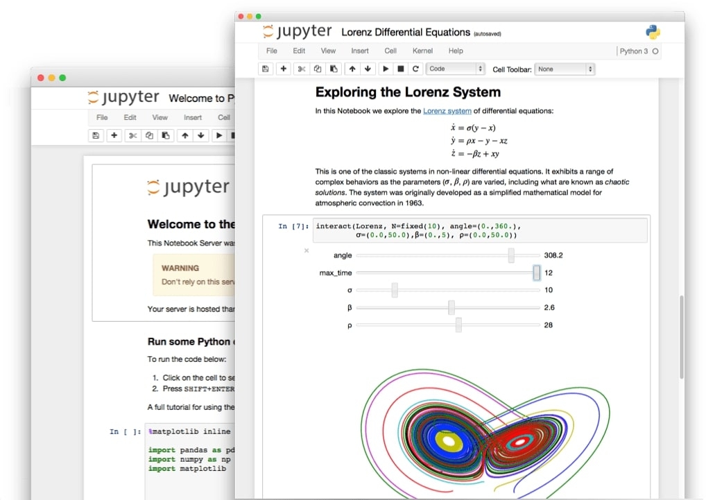
Jupyter is a way to interactively run code (usually Python) directly in your browser. You can split your code into multiple segments, add markdown and display figures inside of your code. This is done with so-called “notebooks”, (.ipynb-files), where your code+text+figures+more are stored. It looks like this:
Why should I use Jupyter?
If you are used to your text editor or IDE of choice you might ask yourself why you should use Jupyter instead of your traditional IDE. I am going to provide you with a few quick reasons as to why you might at least consider Jupyter. If none of these reasons sound appealing to you, then Jupyter might not be for you. Otherwise, I would highly recommend you give it a try! (Maybe it is even integrated in your favorite IDE?)
- The first reason to use Jupyter is that you can dynamically store both code as well as code outputs and visualizations in Jupyter.
Even if we close Jupyter and reopen it, this exemplary plot will still remain in the notebook.
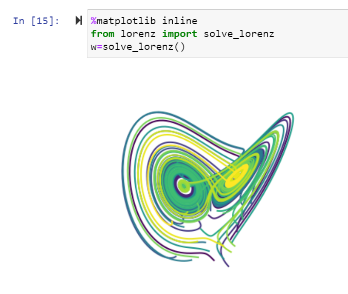
This is awesome for multiple reasons. Firstly you, and everyone who views your notebook can immediately see the result of running your code without having to execute it. This can greatly increase the readability of your code when compared to simple text, because as the saying goes, “a picture is worth a thousand words”. And even if you do not create any visual plots inside of your notebook, seeing the output of your code is incredibly helpful as well.
The second reason is that you can combine Markdown text with your code. With this, you can add helpful comments, headings, rich descriptions, embedded links, images, math equations, and everything else that Markdown allows you to do. This again can make your document a lot more readable and sometimes make your notebook more similar to a code-heavy blog-post than a raw code script. It looks like this:

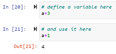
The third reason to consider using Jupyter is that you can split your code into individual cells, execute them separately, but still manage the same global variables. So what this means is that you can put code in one cell and execute just that one cell. Any variables, modules, and everything else that has been loaded or defined globally in this cell, will also be available in every other cell. So if we define a variable a in one cell and inspect the variable of a in another cell (Jupyter automatically prints the output of the last line of code in any cell!), you can see that we do indeed get the correct value for a.
There are a lot more reasons to try Jupyter, such as being able to share your notebooks with other people through tools such as nbviewer or Google Colab, making them able to not only view your notebook, but with Colab also able to run Jupyter for free on a cloud-GPU without having to install any of the dependencies on their own machine! You can also embed interactive widgets in your notebooks, convert your notebooks to a powerpoint-presentation, and much, much more.
How to use Jupyter
Trying Jupyter before installing it
If you want to try out Jupyter in your web browser without having to install anything on your machine, you can! Just experiment with the official examples here or create a notebook in Google Colab. Both are completely free!
Installing Jupyter
Now that you have seen what’s possible in Jupyter, let’s go ahead and install it! Jupyter offers two main development tools: Jupyter Lab and Jupyter Notebook. Jupyter Notebook is exactly what you would expect from the above images, a tool for creating notebooks, i.e. documents that contain code, text, images, and more! Jupyter Lab is an extension of Jupyter Notebook it provides more tools that you would find in traditional IDEs, such as a file manager inside of your code-view, a debugger, an extensions tab, and so on. Below is an image that displays both Jupyter Notebook (left) and Jupyter Lab (right).
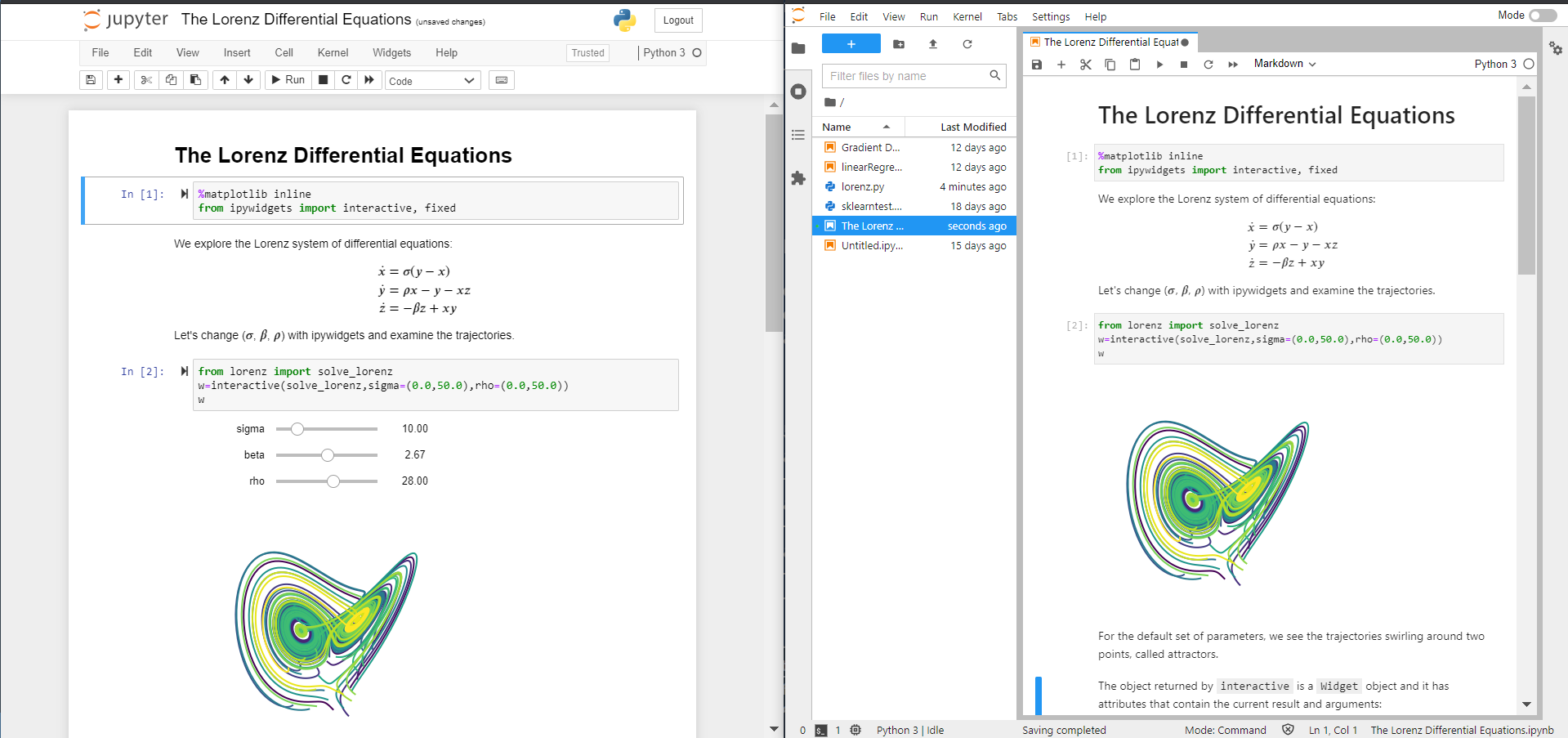
You can think of Notebooks as more of a text-editor and Lab as more of an IDE. You can really try one or both, they are very similar. If you do not have a lot of experience with IDEs or Jupyter in general, I’d recommend starting out with Jupyter Notebook. You can always “upgrade” to Lab if you want to.
To install Jupyter Notebook, you have two main options: pip and conda. If you are unsure whether you should use conda over pip, I recommend you read the article The Only Post you Need to Start Using Anaconda, where you will learn everything you need to know about Anaconda and conda. To install Jupyter Notebook, just run:
pip install notebook #with pipconda install -c conda-forge notebook #with conda
To install Jupyter Lab run:
pip install jupyterlab #with pipconda install -c conda-forge jupyterlab #with conda
You can find more details here.
Starting Jupyter
Once you have installed Jupyter, you can run it via your terminal. Just open up your native terminal
jupyter notebook or jupyter lab depending on which
tool you want to launch. Now a local web server will be started on your machine and you will
be able to connect to Jupyter through your web browser of choice. Usually, you will be able
to access your instance of Jupyter through http://localhost:8888/; the port opened by Jupyter will always be shown to you in your terminal though. If you are using Anaconda Navigator, you can also launch
Jupyter through the Navigator-GUI. To close Jupyter, you should first exit out of Jupyter in your web browser by first clicking on the Jupyter logo in the top left and then clicking the “Quit”-button here:

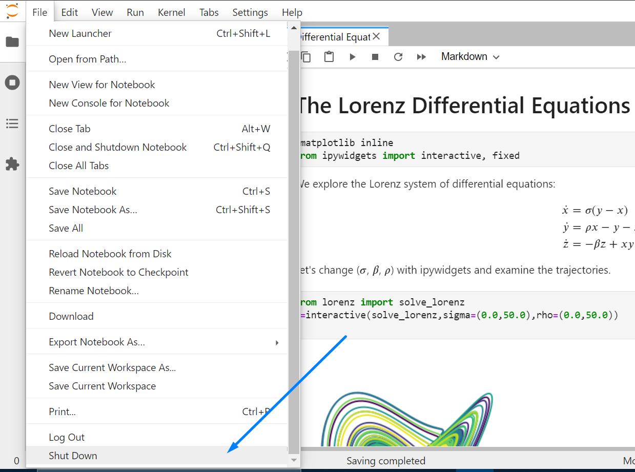
You can also just press Ctrl+C inside of your terminal where Jupyter is running to shut down your local Jupyter-server, but generally, it is recommended to shut down your Jupyter through the web-interface because closing your server by pressing Ctrl+C might result in data loss.
Getting Familiar with the Notebook Layout
One great thing about Jupyter is that you can go through a UI-tutorial directly in Jupyter by clicking on this button here:

Keyboard Shortcuts
If you, like me, enjoy using hotkeys for commonly performed operations, there is good news: Jupyter has plenty of them! You can always pop up the hotkey-menu by pressing “h” on your keyboard while you are not in edit-mode (go through the interface-tour for more info on command- and edit-mode). Below you will find the most important ones.
- Change current mode to command mode: Escape
In command mode:
Change current mode to edit mode: Enter
Change current cell type to markdown: m
Change current cell type to code: y
Insert cell above currently marked cell: a
Insert cell below currently marked cell: b
Cut the currently selected cell: x or dd
Run current cell: Shift + Enter
Focus cell above: Arrow-Up
Focus cell below: Arrow-Down
Select cells: Arrow-Up/Arrow-Down + Shift
Open Command Palette: Notebook: p | Lab: Ctrl + Shift + C
Find and Replace: Notebook: f | Lab: Ctrl + f
I also recommend adding two new hotkeys to move cells around. As far as I know, adding these shortcuts is only possible in Jupyter Lab. You can add shortcuts by going to Settings -> Advanced Settings Editor -> Keyboard Shortcuts or just opening the command palette and searching for “advanced settings editor” and then navigating to the “Keyboard Shortcuts”-Menu. You can add shortcuts for moving cells around by pasting in this piece of code into your custom settings:
{"shortcuts": [{"command": "notebook:move-cell-up","keys": ["Ctrl Shift ArrowUp"],"selector": ".jp-Notebook:focus"},{"command": "notebook:move-cell-down","keys": ["Ctrl Shift ArrowDown"],"selector": ".jp-Notebook:focus"}]}
This will add the following two shortcuts:
- move the selected cells up: Ctrl + Shift + ArrowUp
- moving selected cells down: Ctrl + Shift + ArrowDown
In practice, this will look like this:

Magic Commands
Magic commands are special commands in Jupyter that are prefixed with ”%” or ”%%“. These commands change the way your code is executed inside of Jupyter. Some of the most useful magic commands are listed below.
%time / %%time
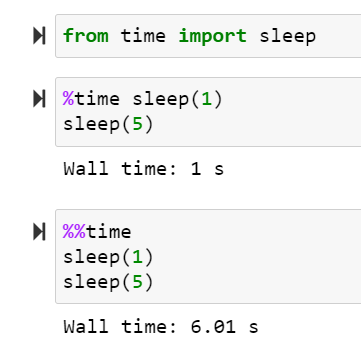
These commands are used to measure how long a specific piece of code takes to execute.
%time (line mode) measures the execution time of one line of code, whereas %%time (cell mode) measures the execution time for one cell.
The cell content is run once and in addition to the expected output you will
also receive the “wall time” (= time spent looking at your wall
%time only measures the wall time
of sleep(1) but not the wall time of sleep(5).
%timeit / %%timeit
This command is similar to the previous one. However, instead of running the current line or cell only once, it is run multiple times. Jupyter executes the cell content n number of times, calculates
the mean time taken and then repeats this process a total of r times.
Then, the average wall time of all repetitions as well as
the standard deviation are calculated and printed. This is useful when your code execution time may vary and
you want to know how much time is taken up in general. Below is an example demonstration.
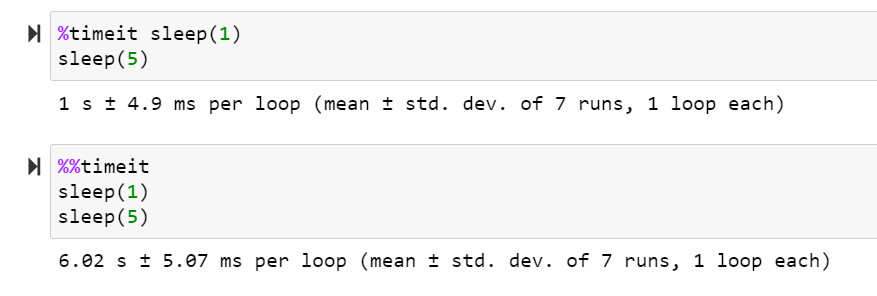
-n and -r-parameter respectively, like this:
%%timeit -n 10 -r 3sleep(0.25)
In most cases though, you will be just fine using %%timeit.
%matplotlib inline
This command makes your matplotlib-plots automatically appear directly in your notebook, without
you having to call plt.show() or a similar command.

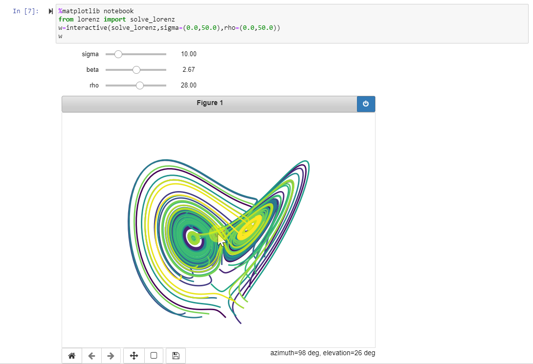
%matplotlib notebook
This is probably my favorite magic command. %matplotlib notebook is similar to
%matplotlib inline, but instead of just displaying an image inside of your notebook,
it instead makes your figure interactive! This is especially useful when you have 3D-plots.
It looks like this:
Autoreload
Autoreload is an extension which automatically updates modules you imported into your Jupyter notebook.
To activate this extension you first have to load it in with %load_ext autoreload and then activate it by running %autoreload 2. So how does it work?
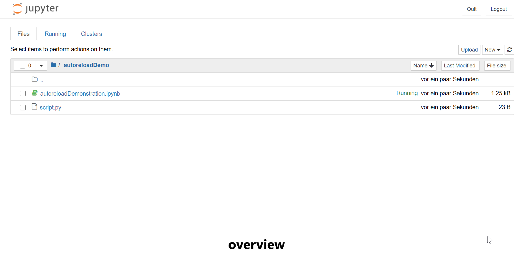
Say f.e. you have a script called script.py which contains a function called foo:
def foo():return 3
You import this function into your notebook like this: from script import foo. Then you change the definition of foo inside of script.py, so that it now returns 5 instead:
def foo():return 5
When you now call foo() inside of your notebook, it will still return the old value of 3. In order for foo to return the new value 5 instead, you would have to restart the kernel and import the function again, meaning you lose all currently active variables inside of your notebook! With autoreload, this happens automatically!
You do not even need to import foo again. Just by calling foo() inside your notebook after it has been updated will automatically update foo. Here is a visual demonstration of autoreload:
You can find more details about magic commands here.
A Note on Importing Scripts
As you may have noticed in the previous section about magic commands and autoreload, to import modules into your Jupyter Notebooks you have to use regular Python scripts. You cannot import other Jupyter Notebooks in the .ipynb-format.
Running Bash or cmd scripts
You can also run Bash or cmd-scripts by prefixing a command with ”!“. So you could f.e. run !ls on Linux or !dir on Windows in a Jupyter cell, which would launch a terminal in your current working directory
!pip install numpy#or%pip install numpy
Customizing your Jupyter with extensions
Jupyter Lab has a great number of available extensions. To search and install packages, all you have to do is go to the extensions-tab and start searching. You can find themes, third-party-integrations for services like GitHub, LaTeX-support, and much, much more!
Jupyter Integrations
If you are lucky, you might not even have to leave your IDE of choice and still harness the flexibility of Jupyter! You can create Jupyter Notebooks directly inside of Visual Studio Code or PyCharm (only the professional edition supports Jupyter). This way you can test the waters without having to install Jupyter directly. With that being said, I’ve tried both the VSCode and the PyCharm integrations and have to say that neither of them convinced me to use leave Jupyter Lab behind. Jupyter Lab feels more fleshed out and it will always have the most recent features since the latest updates will first reach Jupyter directly and only then might be ported to these IDEs. In my own experiments, I have also noticed that PyCharm uses a lot more resources than VSCode, and VSCode starts to lag a bit in larger projects. With Jupyter, I did not have many performance issues until now, so this might also be a point worth considering. For me personally, I will continue using Jupyter Lab. But that does not mean you have to! You can try out the IDE-integrations as well as default Jupyter and see what you like more.
I would love to know whether you prefer the native Jupyter applications or one of the third-party-integrations. If you have a clear favorite, definitely let me know in the comments below!
Further reading
Now that you know everything necessary to hit the ground running with Jupyter, you may want to start working on some real-world projects. For this, I highly recommend that you take a look at my article [currently work in progress], where I go over some great beginner projects that will help you apply fundamental data science and machine learning concepts.
Share on:
