Gradient Descent for Linear Regression Explained, Step by Step

You have most likely heard about gradient descent before. But maybe you still have some questions as to how it really works. Maybe you never found an intuitive and visual explanation for the math behind it, or maybe you never found clean Python code that implements it. If this situation feels familiar, then this article is exactly for you! Here, we’ll go through gradient descent step by step and apply it to linear regression. We’ll take a look at the intuition, the math, and the code behind gradient descent and we’ll also visualize what’s going on under the hood to fully understand this algorithm and learn to use it to it’s full potential.

With that being said, I will assume that you are familiar with linear regression. If you are not, then I would highly recommend you read Linear Regression Explained, Step by Step before coming back to this article. In that article, you will learn everything you need to know about how linear regression works and how you can use it. This post can be considered a sequel to the article about linear regression since I will use some terms and functions that were defined in the post about linear regression. So even if you feel somewhat comfortable with linear regression, I’d highly recommend at least skimming over the linked article.

Since gradient descent is in essence, just math, this post will be more math-heavy than some of my other posts. But do not worry, we will take very small steps and I will make sure to explain every piece of an equation so that you know exactly what we are doing. As long as you know basic high school-level calculus, you are going to be alright. Of course, we are also going to implement gradient descent in raw Python as well as with the help of scikit-learn. And if you have read any of the other articles on this website before, you know that the visual aspect won’t fall short either! So let’s get started!

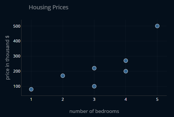
We now want to somehow predict the price of any new house that enters our dataset. To do this, we create a linear function $f(x) = b + mx$ that has a minimal mean squared error (or MSE) with regard to our data points.

Instead of directly computing the ideal values for our variables, we instead approach them step by step. In a nutshell, gradient descent starts with a random function and continuously improves it until it can no longer be improved.

I think Aurélien Géron describes a great analogy for this method in his book “Hands-On Machine Learning with Scikit-Learn, Keras & TensorFlow”, so I will share it with you here.

Imagine you are on the side of a hill and you want to get to the valley. But the air is very foggy. So foggy, that you can only see the ground you are standing on and nothing more. But you can still feel the slope of the hill, right? So by taking very small and cautious steps in the downward direction, you will eventually reach the valley. This is in essence how gradient descent works.

Now let’s apply this to our problem. We can create a three-dimensional plot where we plot the MSE (z-axis) for every $m$ (x-axis) and every $b$ (y-axis). So let’s take a look:

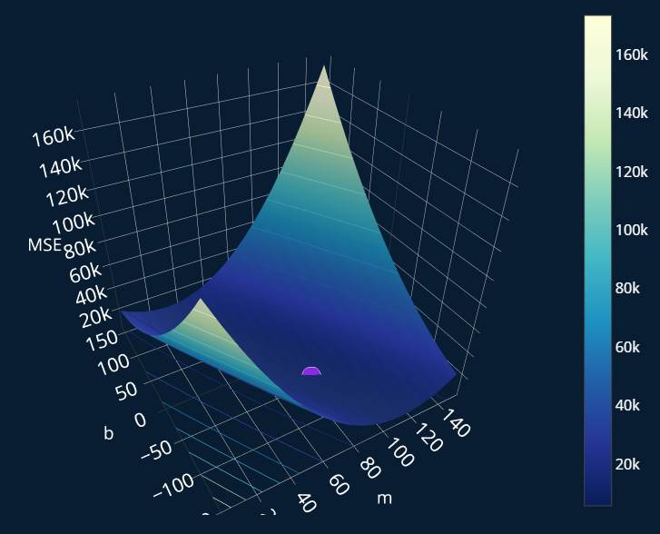
The purple point is the global minimum of our MSE. The question now is, how do we get to this point? We know that we want to approach the minimum iteratively, so our end result should look something like this:

---

1/1

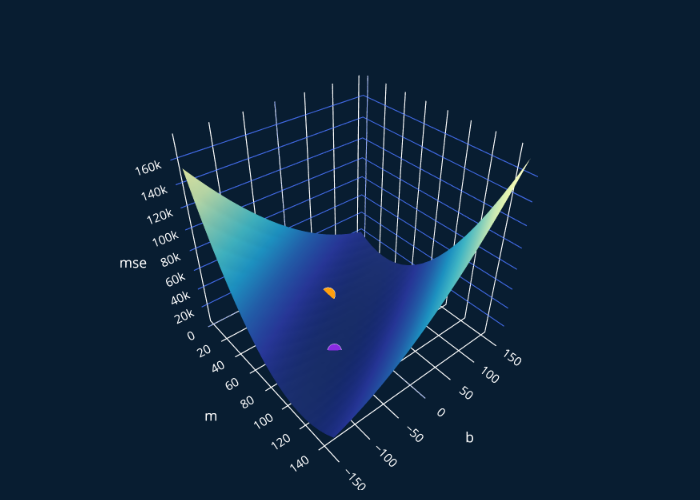
We have now covered the intuition, so let’s now slowly approach the math behind gradient descent.

In other terms, our $m$ is 0 and our $b$ is 0. If we were to plug $f$ into our MSE, we would get:

If we would also plug in our data points, we would get that the MSE for our function $f_0$ is ~$255^2$. This means that the predictions of our function are off by about 255.000$ on average.

Our MSE tells us how well (or rather how poorly) our function fits our data. This means that we want to make our MSE as low as possible. Our MSE is just a function, so if you have taken a calculus class before you might recall that we can compute the minimum of it directly by taking the first derivative of the MSE and setting it equal to 0.

So if we have a function $f(x)=x^2$ we can derive (or differentiate) it once and we get:

This differentiation was done with respect to our variable $x$. This way of writing down the derivative is called Lagrange’s notation, named after Joseph Louis Lagrange. We can also use what’s called Leibniz’s notation, named after Gottfried Wilhelm Leibniz. With this our derivative now looks like this:

With the Leibniz notation, we have to explicitly write out the variable in regard to which we want to derive our function to.

But our MSE depends on two variables, not one. So how can we derive a function with two variables? Well, we can compute what’s called a partial derivative. This sounds fancy but it really just means: treat one variable as a variable and every other variable as a constant.

So if our function looks like this: $f(x,y)=x \cdot y$, we can now no longer calculate just one single derivative. Instead, we can calculate two partial derivatives. One with respect to $x$, and one with respect to $y$. We can write this down like this:

We now use the symbol $\partial$ instead of $d$ to signal that we are taking a partial derivative.

When we differentiate with respect to $x$, we treat $y$ as a constant and vice versa. This is how we can calculate partial derivatives. So let’s now calculate the partial derivatives of our MSE with respect to $m$ and our MSE with respect to $b$.

If you do the math, you will get something along the lines of:

which we can simplify to:

The parts colored in blue are equal to $f(x)$.

What we just calculated is the gradient of our function! The gradient for a function is denoted with the symbol $\nabla$

If we now plug in our values for $m$ and $b$, namely 0 and 0, and we also explicitly write out our data values, we get:

which is equal to:

And with that, we have computed the gradient for our function $f_0$, great! Now that the gradient-part is done, we can move to the descent-part!

The derivative $f'$ of a function $f$ gives us the slope of $f$. In our case, the first value of the gradient (~ -1645) is negative. Ideally, we want this value to be 0, because that would mean we don’t need to move anymore and thus have reached our minimum. Right now this value is negative, which means that the current slope of our MSE with respect to $m$ is negative. This means that to get closer to our minimum, we have to increase $m$. Why? Let’s consider a more simple example.

Imagine we have this simple quadratic function $q(x) = x^2$, which looks like this:

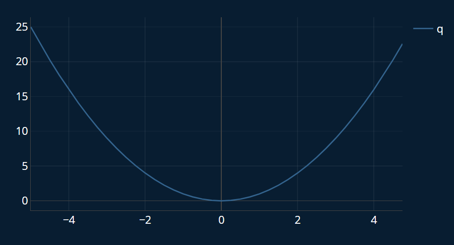
Now we want to find its minimum. We derive the function and we get $q'(x) = 2x$. There is only one derivative because we only have one variable. Now we can overlay $q$ and $q'$. Let’s imagine $q$ as our imaginary “2D-hill” for a moment, and choose a random starting position, like this one:

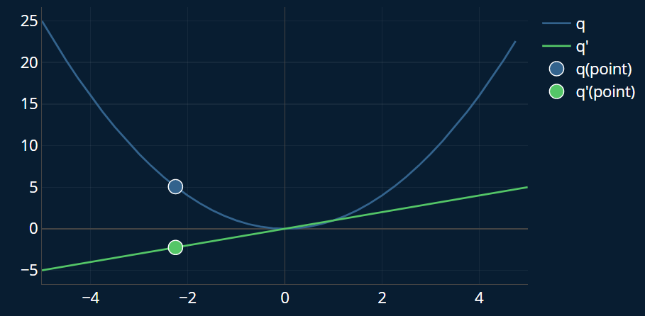
Ok, so how do we know which direction we need to move towards to reach the minimum of our simplified “2D-hill”? Our derivative at this point is -2.25.

Our minimum is at the point where our derivative is zero, i.e. the point where $y=0$. So we always want to go towards this point.

If we move towards the right, i.e. if we increase $x$, we get closer to the point where $y=0$. If we would be standing on the opposite side of our hill, our derivative would be positive. In that case, we would have to decrease $x$ to get closer to our minimum.

So for every point on the green line (the derivative), if it is below 0 (i.e. if our derivative is negative), we have to increase our variable. And if it is above zero (i.e. our derivative is positive), we have to decrease it. In other words, we just subtract our derivative from our variable. If our derivative is negative, the minuses will cancel out and it will be added instead.

But our derivative not only tells us which direction we should move towards, it also tells us how large our steps should be. If the absolute value of our derivative is high, meaning it is high in the negatives or high in the positives, then our steps can be larger. Similarly, if our derivative is close to zero, we will only perform small steps. In other words, if the slope below our feet is very steep, we can cover more distance with a single step than if our slope was very shallow.

We can draw imaginary arrows to visualize the direction and size of our steps at any point based on our derivative:

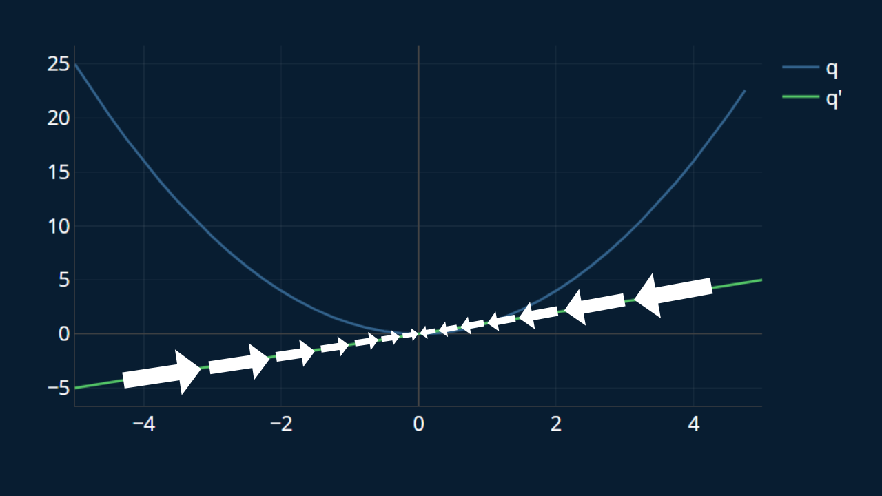
So the important points to remember are:

• positive derivative -> reduce
• negative derivative -> increase
• high absolute derivative -> large step
• low absolute derivative -> small step

Now let’s go back to our original example.

In the case of our gradient, the first value tells us how to adjust $m$ and the second one tells us how to adjust $b$. Let’s first recall the visualization of the MSE (our “hill”) and let’s also add in the point we are currently at as well as the minimum:

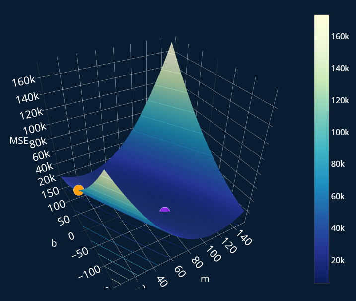
Great! The orange point displays our current position. Now we can visualize the partial derivative of our MSE with respect to $m$ in the same way, and we will also display our two points as well:

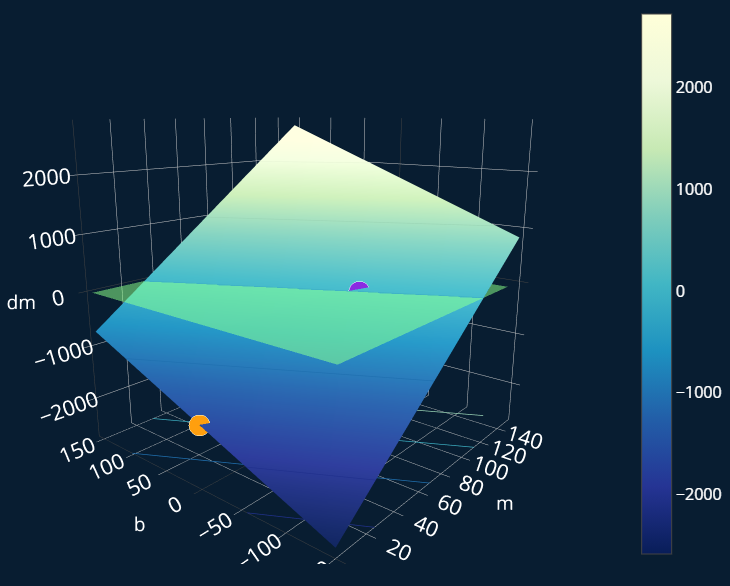
As you may notice, this looks very similar to our simplified example with $q$ and $q'$! Here we have three variables, so we want to get to the “point” where $z=0$. But because we are in three dimensions, there isn’t just one point where this is true, there is an entire plane where $z=0$. So to make the plot a bit easier to interpret, I also added in a greenish plane at $z=0$.

We can now apply the same logic we used in our 2d-example. Currently, we only care about adjusting $m$. So for every point on this plane, if it is above this slightly transparent greenish plane, we need to decrease $m$. Similarly, if it is below the plane, we have to increase $m$. We can once again draw our imaginary arrows to visualize the direction and size of our steps:

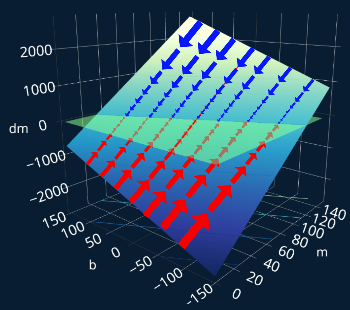
As you see, right now we only move across the x-axis (or in our case, the $m$-axis), because we only want to know how we need to adjust $m$.

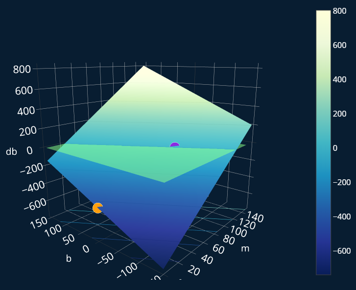
We can also create a similar 3d-plot for the partial derivative of our MSE with respect to $b$ to see how we need to adjust b:

And we can again draw some imaginary arrows to visualize the steps we would have to take at any particular point:

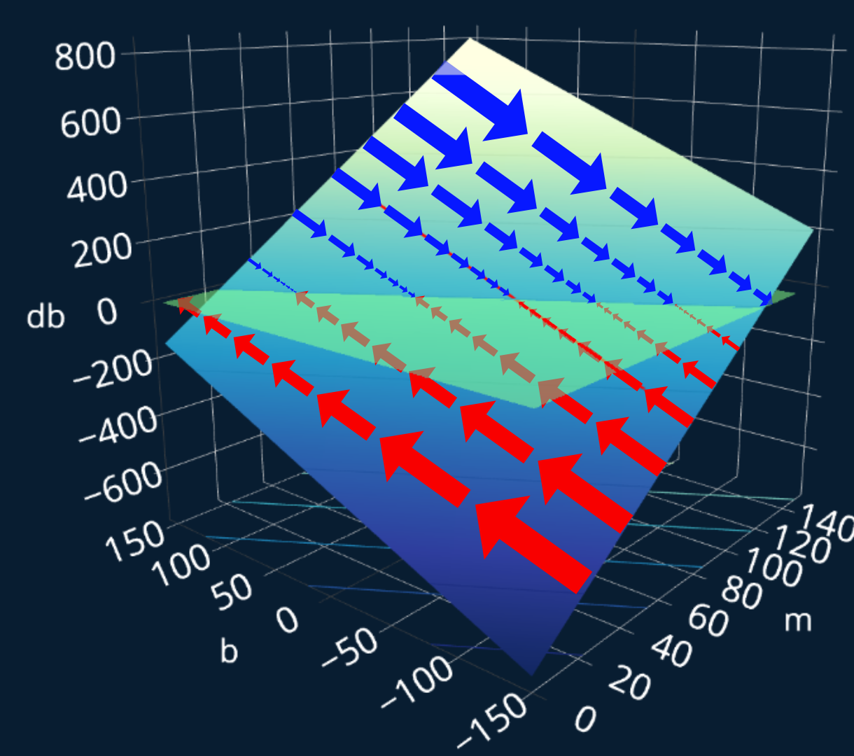
This again looks very familiar. Our gradient was this:

so now we know that we need to increase both our $m$ and our $b$. But we need to increase our $m$ a lot more than we need to increase our $b$! This makes sense because the slope of our “MSE-hill” at our current point is steeper in the $m$-direction than it is in the $b$-direction. If you have been following this post very closely, you might notice that something is off.

Let’s see how our step would change our position on the hill:

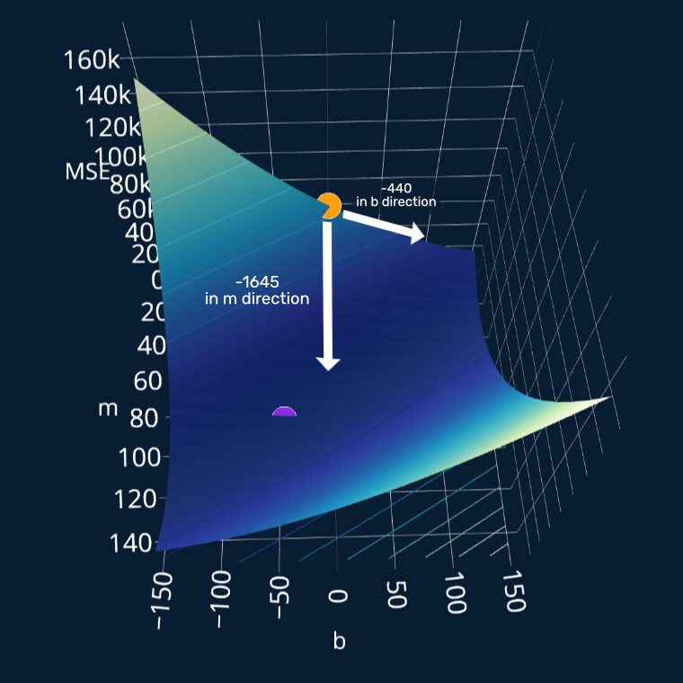
Indeed, the slope in $m$-direction is steeper than the one in $b$-direction. And indeed, the arrow in $m$-direction leads us towards our minimum. But wait! The arrow in $b$-direction leads us away from our minimum! What?! Have we done something wrong? Isn’t gradient descent supposed to take us to the minimum, not away from it? Well, no, we did not do anything wrong and yes, gradient descent seems to take us in the wrong direction. But our derivatives are correct and we have also not made any other mistakes up until this point. But why are we moving in the wrong direction, then?

Let’s take a closer look at the slope in $b$-direction. It really does look like it is leading down towards the right in the above image. Meaning there could be a minimum there. Gradient descent just doesn’t know if there is one. Right now, it seems like a valid option because the slope points us towards this side of the plot. But once we perform a couple more steps of gradient descent, we will soon see that the slope in $b$-direction begins to change and we do indeed “turn around” and start moving in the right direction again. So right now there isn’t really anything we can do to “correct” our movements, because we don’t know where the minimum really is, or at least, our program does not know so. Only we have this fancy 3d-visualization where we can see that we are moving in the wrong direction. But gradient descent does not see the issue, at least not now. In our case, this is no big deal. We only have one minimum, which means that we will find it sooner or later. But in scenarios where we have more than one minimum, gradient descent can actually get stuck in a local minimum, and not get out. But this is beyond the scope of this article. For now, everything is alright and we will soon see that gradient descent will still find our minimum, it might just need a few extra steps to do so.

Ok, so we now understand how and why we need to adjust our parameters. But by how much should we adjust them? Should we really increase our $m$ by 1645? No, that would be way too much! If we were to increase our $m$ by 1645, we would completely overshoot our minimum and land on the other side of our plot. Instead, we choose a so-called learning rate. Our gradient is then multiplied by our learning rate before we apply it to our parameters. This learning rate is a number between 0 and 1. 0 means we do not change our values at all and 1 means we subtract the entirety of our gradient. Common values for a learning rate are usually in the range of $1e-3 = 0.001$. If we choose a learning rate of 0.001, we would update our values like this:

Our new values would now be:

So we update our function:

We can add a little $_1$ at the bottom to show that this is our function after one iteration of performing gradient descent.

If we calculate the MSE for our new function, we get ~62362.30 $\approx$ $249^2$! It’s improved (before it was ~$255^2$)!

Now we do this over and over again until we cannot improve our MSE any further. In practice, you will almost never achieve an MSE of 0, so it’s a good idea to look at how much our MSE improves every iteration, and once we make little to no improvements, we can usually stop. This technique in particular even has a name and it’s called early stopping.

We have now learned how the math behind gradient descent works and how we can start with some random function and iteratively improve it until we end up with our ideal function. Now, let’s also implement this algorithm in Python.

In essence, we want to define a function gradient_descent that takes in our data ($x$ and $y$), our variables ($m$ and $b$), our minimization criterion (in our case this will be the MSE, since we want to minimize that) and performs gradient descent to find the values for our variables that minimize the criterion. We also need to pass in a learning rate and the number of iterations (commonly called epochs) we want to perform gradient descent for.

 dataset = np.array([
     (1,80),
     (2,170),
     (3,100),
     (3,220),
     (4,200),
     (4,270),
     (5,500)
     ])
 
 x = dataset[:,0]
 y = dataset[:,1]
 
 def add_intercept_ones(X):
     intercept_ones = np.ones((len(X),1)) # results in array( [ [1],..,[1] ] )
     X_b = np.c_[intercept_ones,X]
     return X_b
 
 X_b = add_intercept_ones(X)

Since we could have more than just one feature (the number of bedrooms), we might have a function with more variables. If we wanted to predict the price of a house based on the number of bedrooms, the year it was built in and the average house price of the city the house stands in, our function would look more like this:

To make our life easier, we will vectorize our function and instead write:

If you are asking yourself where the $+ b$ went, what this ”$_b$” in $X_b$ means, or if our function really remained the same, I encourage you to read the section about vectorization in the post about linear regression, where I explain this step in a lot more detail.

So the skeleton of our function should look something like this:

 def gradient_descent(x, y, theta, criterion, number_of_iterations, alpha):
     for i in range(number_of_iterations):
         # perform one step of gradient descent
 
     return ideal_theta

We want to perform number_of_iterations many gradient descent-steps, which is why we added the for-loop. Now let’s perform gradient descent step by step.

First, we have to calculate the predictions of our model for $\textbf{X}_b$. We can do this by defining a higher order function that takes in $\textbf{X}_b$ and $\boldsymbol{\theta}$ and creates our linear function for us, which it then returns. This would look like this:

 def create_function(theta):
     def f(X_b):
         return np.dot(X_b,theta)
 
     return f

We can then use our function like this:

 f = create_function(theta)
 y_predicted = f(X_b)

Note that we could also just write np.dot(X_b,theta) directly, instead of creating this higher order-function, but this way we can more easily reuse our code if we wanted to create a more complicated function.

And now let’s translate it into (vectorized) code:

 def mse(y, y_predicted):
     error = y-y_predicted
     loss = 1/(y.size) * np.dot(error.T, error)
     return loss

Note that since error is just a vector containing all of the residuals, np.dot(error.T, error) is just a shortcut for the dot product of error with itself. This results in the same output as if we were to calculate each residual individually, square them up and add them together. If you are still unsure about this, I recommend you implement this function both vectorized and non-vectorized and then compare them to each other.

Now we can calculate our loss like this:

 loss = mse(y, y_predicted)

The last step which we have to perform is to optimize our variables. First, we have to compute the gradient of our MSE. For this, we need our two partial derivatives. Let’s recall what they look like:

We can implement our derivatives like this:

 def mse_derivative_m(X,y,y_predicted):
     return -(2/y.size) * sum(X * (y - y_predicted))
 
 def mse_derivative_b(y,y_predicted):
     return -(2/y.size) * sum(y - y_predicted)

Now we can compute our gradient in just one line of code:

 gradient = [mse_derivative_m(x,y,y_predicted),
             mse_derivative_b(y,y_predicted)]

Once we have our gradient, we can adjust our $m$ and our $b$:

 m -= learning_rate * gradient[0] #adjust m
 b -= learning_rate * gradient[1] #adjust b

Let’s now put all of this into our main function:

 def gradient_descent(x, y, theta, criterion, number_of_iterations, learning_rate):
     X_b = add_intercept_ones(X)
     for i in range(number_of_iterations):
 
         # predict and calculate loss
         f = create_function(theta) # create the current function
         y_predicted = f(X_b) # predict our entire x
         loss = criterion(y,y_predicted) # calculate the error
 
         # perform optimization
         gradient = np.array([mse_derivative_b(y,y_predicted), mse_derivative_m(x,y,y_predicted)]) # calculate gradient
         theta = theta - learning_rate * gradient #adjust m and b
 
     return theta

Great! Let’s try it out:

 theta = np.array([0.,0.])
 num_epochs = 25
 learning_rate = 0.001
 ideal_theta = gradient_descent(X, y, theta, mse, num_epochs, learning_rate)

If we then inspect our ideal theta we get:

 >>>print(ideal_theta)
 array([ 8.19030548, 31.03371126])

It’s certainly getting closer to our minimum! Our minimum lies at the point where and $b=-46.316$ and $m=84.737$. As you see, $m$ is moving in the right direction, but $b$ is still moving the wrong way.

We can now calculate the MSE for our ideal function:

 ideal_function = create_function(ideal_theta)
 y_pred = f(X_b)
 print(mse(y,y_pred))

which returns us a value of ~23223 $\approx$ $152^2$! Awesome! But it’s not exactly at the minimum yet. If we adjust our learning rate a bit and train our model longer, we do eventually reach the minimum. F.e. with a learning rate of 0.075 and 200 training epochs, we reach a loss of ~5692, which is very close to our minimum. Feel free to experiment with the values a bit and see if you find a more optimal configuration. If you do, definitely let me know in the comments below!

Let’s now make a few improvements to our function. Wouldn’t it be cool if we could track the loss of our function across every epoch? We can do this by creating a new list and always appending the current loss to it. Also, we can print the current loss every 10 or so epochs!

 def gradient_descent(x, y, theta, criterion, number_of_iterations, learning_rate):
     X_b = add_intercept_ones(X)
     loss_history=[]
     for i in range(number_of_iterations):
 
         # predict and calculate loss
         f = create_function(theta) # create the current function
         y_predicted = f(X_b) # predict our entire x
         loss = criterion(y,y_predicted) # calculate the error
         loss_history.append(loss)
 
         # perform optimization
         gradient = np.array([mse_derivative_b(y,y_predicted), mse_derivative_m(x,y,y_predicted)]) # calculate gradient
         theta = theta - learning_rate * gradient #adjust m and b
 
         if i%10==0:
             print("Current Epoch: {}, Current Loss: {}".format(i,loss))
 
     return theta,loss_history

We now execute gradient descent once again:

 theta = np.array([0.,0.])
 num_epochs = 200
 learning_rate = 0.0075
 ideal_theta, loss_history = gradient_descent(X, y, theta, mse, num_epochs, learning_rate)

Now we can plot our loss across the iterations:

 import matplotlib.pyplot as plt
 plt.plot(np.arange(num_epochs),loss_history)

which gives us the following plot:

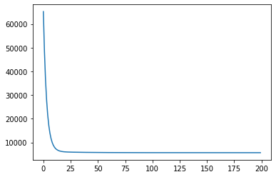
Nice!

If you want to add some additional features to the implementation, here are a few ideas:

• Return the history of thetas in addition to the history of losses
• Add functionality to save/load your (ideal) function
• Implement early stopping

If you want to make sure you understood everything in this article, try to implement one or two of these features!

We can also use the popular library scikit-learn to solve our linear regression problem using gradient descent. For this, we can use the SGDRegressor-class. Scikit-learn expects our x to be two-dimensional (since, in most cases, we will have more than one feature), so we’ll also redefine our x to be two-dimensional: The code looks like this:

 X = np.array(
     [
             [1], [2], [3], [3], [4], [4], [5]
     ]
 )

Then, we use the SGDRegressor-class like this:

 from sklearn.linear_model import SGDRegressor
 sgdreg = SGDRegressor(learning_rate="constant",eta0=0.0075,max_iter=200,random_state=42) #eta0 is our initial learning rate
 sgdreg.fit(X,y)

And we can then inspect our parameters like this:

 >>>print(sgdreg.coef_,sgdreg.intercept_)
 [68.95520002] [12.285233]

Now you might notice that this variant does not directly converge to our minimum, which is because scikit-learn does a bit more under the hood than our own implementation. It may look like our implementation is faster, but in truth scikit-learn’s implementation is a lot more general and implements a variety of other aspects like a regularization term to reduce the risk of overfitting. Apart from that scikit-learn starts with random values for the parameters instead of starting with 0, which has some benefits, but in this particular case can result in more epochs being needed to reach the minimum. But this article is getting pretty long and I don’t want to make this even longer, so for now, this should suffice. If you want, you can also play around a bit with the individual parameters and see which ones have the strongest effect on the final model parameters.

Now that we have covered gradient descent in detail, let’s have some fun and look at a complete visualization of the process, shall we? We can visualize the MSE as well as our function and both partial derivatives for every epoch. As you may have noticed from the loss history above, the loss takes a deep dive in the first few epochs and then decreases only slowly. So to keep the visualization fluid, I will show the first 10 epochs and then only every 15th epoch after that. We will display our current function/state at that particular epoch with the familiar orange and the optimal point in a familiar purple. Putting all this together, we get:

---

1/18

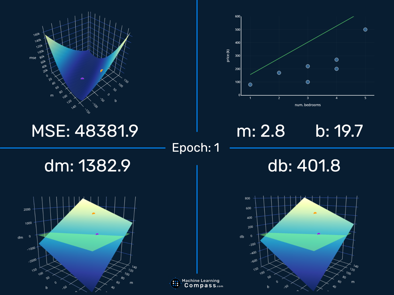
Cool! Now you might notice a few things in the top left animation.

First of all, our point seems to jump around a bit too much. It first starts off “to the left” of the minimum, then jumps and is then located to the “right of it”, then it again jumps to the left side, and so on. When we created our initial visualization in the section The Intuition, this process looked a bit cleaner and our orange friend did not jump around this much.

Usually, this “jumping around” is not what we want. This is a clear sign that our learning rate is too high and our parameters may overshoot the minimum. In our particular case, this does not end up being a big problem, because our function still gets to our minimum pretty quickly. However, if we were to just sliiightly increase our learning rate, say to 0.08, we would get a problem. Because in that case, we overshoot our minimum so much that we actually end up “jumping out” of it:

---

1/1

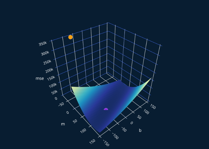
At this point, you might ask, “so how can we pick a good learning rate?“. Great question! In fact, this is such a good question that I decided to dedicate an entire post to answer this question and go over the different techniques to choose and adapt your learning rate, and look at the effects different learning rates have on your model. I highly recommend you read that article after reading this one, it blends in really well with the content from this post!

With this, you have now learned how to use gradient descent to iteratively solve linear regression. We’ve looked at the problem from a mathematical as well as a visual aspect, and we’ve translated our understanding of it into working code, once using just Python and once with the help of scikit-learn. If you have any feedback on this post, I’d love to hear your thoughts in the comments below! These articles take many hours to create and it makes me truly happy to see people give both praise and critique so that I can make sure these posts do their intended job well: help you become better at machine learning!

If you’ve made it to the end, good job! Pat yourself on the back, you deserve it. Gradient descent surely isn’t the easiest algorithm in machine learning, but if you approach it step by step it is a lot less scary than only seeing the final equation with no explanation.

If you can’t get enough of linear regression, I recommend you read the post Lasso and Ridge Regression Explained, Step by Step next, where you will learn everything about lasso and ridge regression, which are variations of linear regression that solve some of the issues vanilla linear regression has.

If you are more interested in gradient descent and want to continue right where this post ends, you should read the article How To Choose Your Learning Rate, where we will take a detailed look at the issues we saw at the end of this article. You will learn about all of the different techniques for choosing and adapting learning rates, so you’ll never have to worry about picking random learning rates again!