Ridge Regression Explained, Step by Step
Ridge Regression is an adaptation of the popular and widely used linear regression algorithm. It enhances regular linear regression by slightly changing its cost function, which results in less overfit models. In this article, you will learn everything you need to know about Ridge Regression, and how you can start using it in your own machine learning projects.
Share on:
Background image by Jeremy Bishop (link)
Outline
You have probably heard about linear regression. Maybe you have even read an article about it. Lasso and ridge regression are two of the most popular variations of linear regression which try to make it a bit more robust. Nowadays it is actually very uncommon to see regular linear regression out in the wild, and not one of it’s variations like lasso and ridge. The purpose of lasso and ridge is to stabilize the vanilla linear regression and make it more robust against outliers, overfitting, and more. Lasso and ridge are very similar, but there are also some key differences between the two that you really have to understand if you want to use them confidently in practice. This is why, starting with this article, we’ll take a deep dive into ridge and lasso regression! In this article, you will learn everything you need to know to start using ridge regression in your next machine learning project. First, we will look at a problem that may occur with regular linear regression, overfitting, and then we’ll explore ridge regression mathematically, visually, and code it up in raw Python as well as with scikit-learn. Let’s start!
Prerequisites
This article assumes that you are already familiar with linear regression. If you are not, I very highly recommend that you read Linear Regression Explained, Step by Step prior to reading this article. If you are unfamiliar with linear regression, this article might be very difficult to understand. This article can be considered a follow-up to the article about linear regression, so reading this post will be much easier if you’ve read the one about linear regression as well. Two other posts that will be very helpful for understanding this particular article are Bias, Variance, and Overfitting Explained, Step by Step as well as How to Split Your Dataset the Right Way. In the first article, you will learn all about overfitting, and how it can be explained using the notions of bias and variance. Overfitting is one of the reasons ridge and lasso exist in the first place, so understanding it will make this post a bit easier to digest. The second article will teach you all about how you can split your dataset into a training and testing portion. We’ll perform this splitting in this post as well, so it won’t hurt if you understand why exactly this is useful. You don’t have to read these two articles before this one, but they will make reading this post about ridge regression easier, and clear up some confusion you might have about certain sections. With that being said, let’s take a look at ridge regression!
The Problem
So what is wrong with linear regression? Why do we need more machine learning algorithms that do the same thing? And why are there two of them? Let’s explore these questions in more detail.
The goal of linear regression is to fit a line to a dataset in such a way that it minimizes the mean squared error of our line and our data. With regular linear regression, we don’t tell our model anything about how it should achieve this goal. We just want to minimize the MSE and that’s it. We don’t really care whether the model parameters in our model are very large or very small, we don’t care about overfitting, and so on.
To make the distinction between linear regression and ridge regression more clear, we will from now on use the term OLS regression (or ordinary least squares regression) to describe the “normal” linear regression we already know.
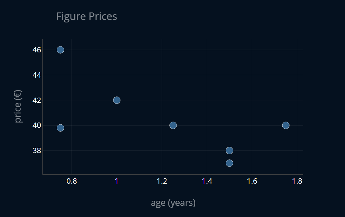
But you might say, OLS regression is not that complicated, what could go wrong with such a simple model?, which would be an excellent question to ask! So let’s look at a case when things don’t go as planned. Imagine we have a very small dataset, containing figure prices. Each entry in the dataset contains the age of the figure as well as its price for that age in € (or any other currency). We now want to predict the price of a figure, given its age, using linear regression, to see how much the figures depreciate over time. The dataset looks like this:
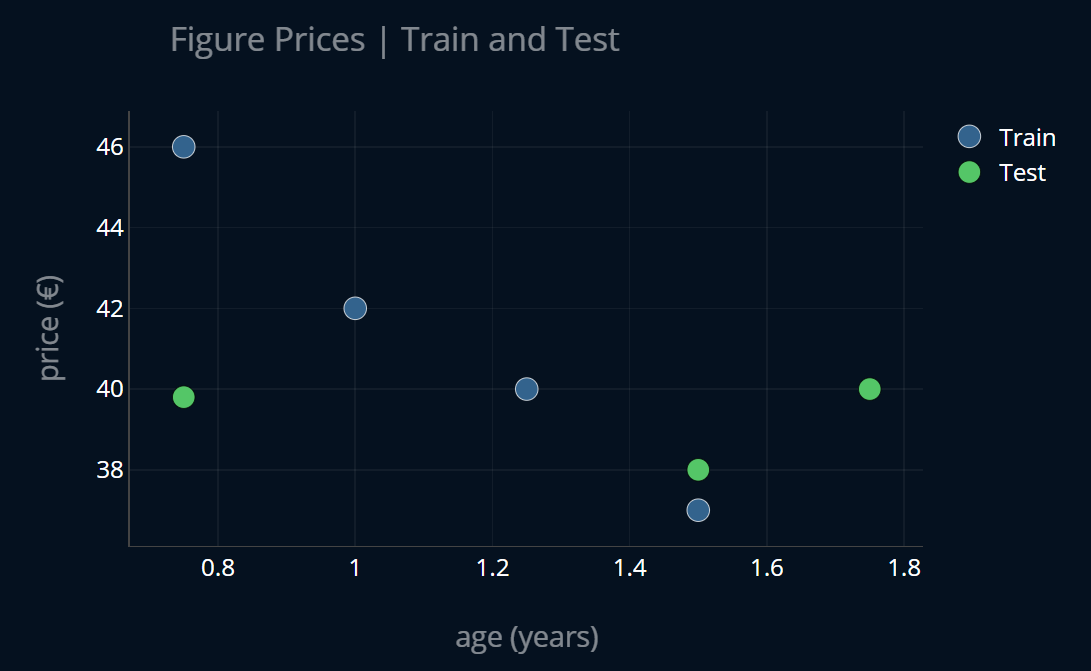
If you’ve read the article How to Split Your Dataset the Right Way, you know what we’re going to do next. That’s right, we’ll split our dataset into a train set and a test set! The partitioned dataset looks like this:
We now perform linear regression on the training data. Let’s plot the resulting linear function alongside our partitioned dataset:
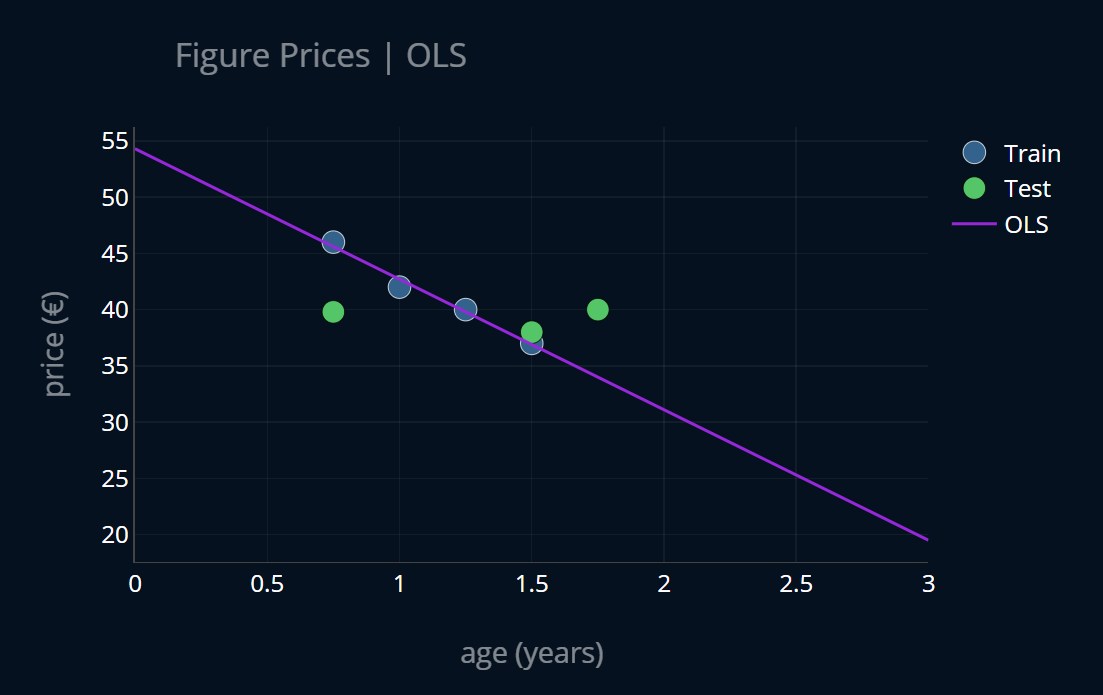
Now I don’t know about you, but the function generated by our linear regression model does seem to have a pretty steep slope. A one-year-old figure worth 40€ would be worth only 20€ after three years, according to our function. That doesn’t seem right! If you’ve read the article about bias and variance, you know how to describe this model. It has a low bias and a high variance and is therefor overfit. We can confirm this by looking at the training and testing errors
mse is the mean squared error which we’ve first implemented in the article about linear regression
and then implemented it more efficiently in the article about vectorization.mse(y_train, ols.predict(X_train))# output: 0.175mse(y_test, ols.predict(X_test))# output: 23.616666666666653
But how can we create a better model, one that is not overfit? And what exactly leads to our model overfitting?
Improving OLS Regression
Let’s first try to come up with an “imaginary” model that is a better version of our current one and one that isn’t overfit. Let’s try and create a plot of our idealized model and display it alongside our current model. The result looks like this:
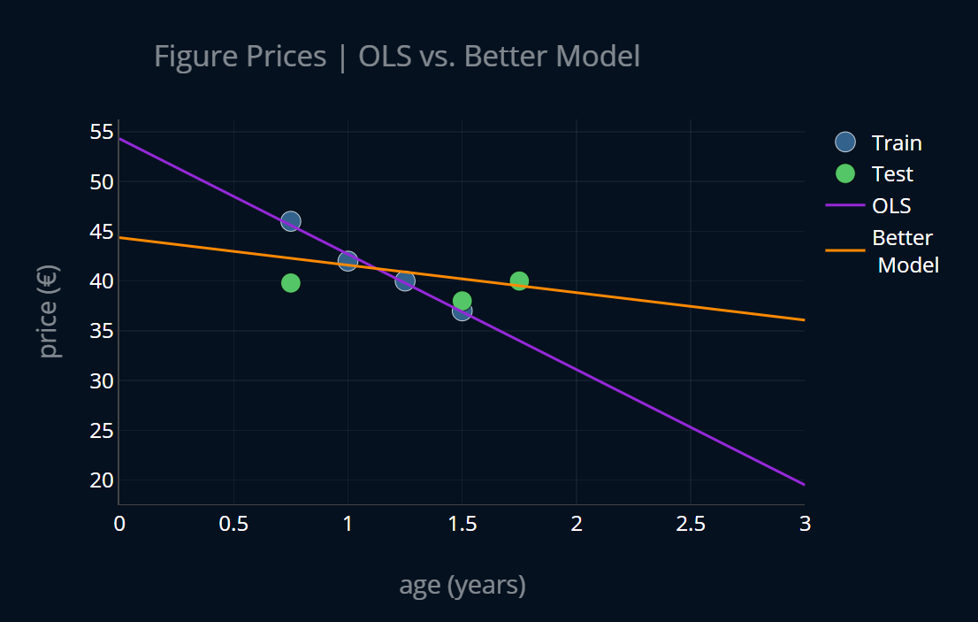
Alright, that looks better! Our idealized model does seem to have a slightly higher bias than our OLS model, but it also has a lot lower variance. We can confirm this by looking at the MSE of both models on the training and testing data and then compare the relative difference of the errors for training and testing, which, as we know from the article about bias and variance, is a good measure to intuitively get a feel for the variance of a model. If we do this, we get the following results:
| MSE (Train) | MSE (Test) | R.DIFF | |
|---|---|---|---|
| OLS | 0.175 | 23.62 | 13397.14% |
| Imaginary model | 6.28 | 3.77 | 50.2% |
With this, we can confirm our assumption. Our imaginary model does have a larger bias, but its variance is very low, in contrast to our OLS model. But what exactly is the difference between our OLS model and our new, imaginary model? Let’s inspect the two functions that were generated by our two models. We will write down the linear functions and :
f
What we can see is that the (absolute) model parameters of our OLS model are larger than the parameters of our imaginary model. In fact, the first parameter differs by around 320\% between the models! So our findings suggest that the cause for our OLS model overfitting are large model parameters. Maybe, if we somehow force our model to generate smaller parameters, we can achieve better results and generate a model that looks more like our imaginary one? Let’s try this out and see how it goes.
Regression With a Twist
Ok, so we’ve said that we want to force our model to generate smaller model parameters. How can we do that? Pause for a second and see if you can find a way in which we can achieve this, without changing up our model too much. Got an idea? How does our model know what model parameters it should generate? How does our model know what good parameters are and what bad parameters are? It gets this information from our loss function. Currently, our loss function is the MSE. Recall what it looks like (n is the number of samples in our dataset):
If this definition does not look familiar to you, but this one does ( and are just the data points of our dataset):
then I recommend you take a look at the article Vectorization Explained, Step by Step, where we take this familiar definition and transform it into the vectorized form above, which can be computed significantly faster
This MSE is the function that we, or rather, our model, is trying to minimize. Right now, it only contains the mean sum of squared residuals. But if we add another term to this function, our model will then have to minimize both the mean sum of squared residuals, as well as our additional term at the same time. Let’s call this additional term penalty. So which penalty do we add? We know that we want to minimize our model parameters, and our model minimizes the loss function, so let’s just add the model parameters into the equation, shall we? Our model has parameters (intercept) and (slope), so let’s add them to our loss like this:
More broadly, if we have model parameters, our new loss will be:
Ok! There’s just one problem. Since our model parameters can be negative, adding them might decrease our loss instead of increasing it. We encountered a similar problem when we built linear regression in Linear Regression Explained, Step by Step. In order to circumvent this, we can either square our model parameters or take their absolute values. In this post, we’ll only take a look at the square of the sum of model parameters.
We can vectorize our new loss function since the last part is just the dot product of our parameter vector with itself:
If you are unsure about this, just quickly make an exemplary calculation and confirm that this really does not change our loss function. If you are familiar with norms in math, then you could say that this new loss contains a squared -norm (or Euclidian norm), This is also the reason why this term is sometimes referred to as an L2 regularization. This means that we can rewrite our new loss like this (a norm is denoted using two vertical lines, like this: ||):
Now, let’s perform one final change. Right now, we can’t control how much the model parameters should be factored into the equation. We want our model to minimize the MSE and the model parameters, but maybe one is more important than the other in a particular case? What if we want our model to focus most of its attention on the MSE and only pay a small bit of attention to the model parameters? To be able to control how much our new penalty term weighs into the equation, let’s add an additional parameter
Ok, enough math for now. Let’s solve the mystery and stop calling this metric new loss. What you see in front of you is exactly the loss function of ridge regression!
OLS vs Ridge
With the intuition and math now covered, let’s try to visually grasp the fundamental difference between OLS and ridge. More specifically, let’s try to understand the difference between the two by looking at how strongly these models react to change in data. Since ridge has a penalty term in its loss function, it is not so sensitive to changes in the training data when compared to OLS regression, because ridge has to make sure that the penalty term stays small. However, OLS regression has no penalty term, which means that it will minimize only the MSE, with disregard to the size of its model weights. So what this means intuitively is that, if we slightly change our training data, our ridge model might only change its parameters a little bit, while our OLS model parameters will change a lot more. Let’s take just two data points and see how our two models change when we slightly shift the position of our data points. Below you can find a plot that shows the OLS model for the two data points. At the top of the plot, there is a button which you can press to slightly shift the data points across the x-dimension. After each press, a new OLS model will be displayed, while the old model will take on a more transparent tone. Press the button a couple of times and notice how (strongly) the functions differ from each other.
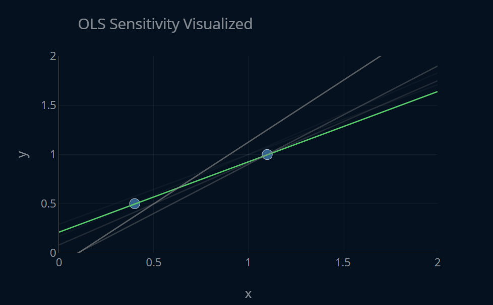
We can see that even if we only change our data points by just 1 point in the x-direction, our OLS model does change its shape quite a bit. Let’s create this same plot once more, but this time with ridge regression. Try to compare the functions generated by ridge to the ones generated by OLS.
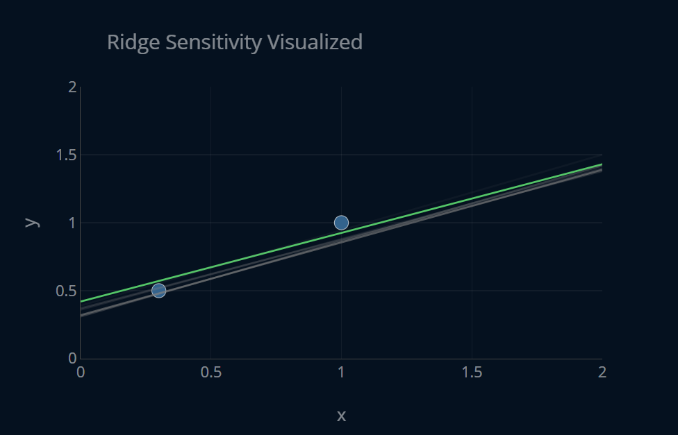
Ok, there’s clearly a difference there! We can see that the functions generated by ridge vary only slightly in their parameters, while the functions generated by OLS differ a lot more. We can see how ridge is less sensitive to changes in the input data than OLS regression. Therefor we can conclude that ridge models have a lower variance than OLS models. However, because of the penalty term, they usually have a slightly higher bias than OLS models.
Solving Ridge Regression
We have now talked at length about ridge regression and how it differs from OLS regression. But how can you actually determine the model parameters ? Just like with linear regression, we have a variety of methods at our disposal! The good news is that we can solve ridge regression with the same methods and techniques we used to solve OLS regression! These were 1. solving the normal equation and 2. using gradient descent. Let’s look at both options!
Normal Equation
The good news here is that there is a normal equation for ridge regression. Let’s recall how the normal equation looked like for regular OLS regression:
We can derive the above equation by setting the derivative of the cost function of linear regression (the MSE) equal to zero and solving for our model parameters. We do the same thing for ridge regression. Our loss looks like this:
We now differentiate this function, set it equal to zero, solve for and we get:
where is an identity matrix with dimensions
As with the normal equation for linear regression, the solution to this equation gives us the ideal parameters for our directly, in one step. If you’ve read the section about complexity in the article about linear regression, then you’ll know that solving the normal equation is your best bet in most cases. However, if you have a very large number of features, you might be better off using an iterative algorithm, like gradient descent. Let’s take a look.
Gradient Descent
Alternatively to solving the normal equation, we can differentiate the ridge cost function to obtain its partial derivatives (i.e. compute its gradient) and then perform gradient descent to iteratively approach the optimal solution. If you are interested in learning about how gradient descent works and how you can implement it in raw Python as well as with scikit-learn, I recommend that you read the article Gradient Descent Explained, Step by Step, where you will learn how to do exactly that. The implementation of gradient descent for ridge regression is very similar to gradient descent for linear regression, and in fact the only things that change are how we compute the gradients and our loss function.
Implementing it in Python
Now that we’ve briefly looked at the two main methods of solving ridge regression, let’s also implement them in Python! First we’ll implement it from scratch and then we’ll look at how we can make our lives easier by using scikit-learn.
Implementing the Normal Equation
Similar to the normal equation for OLS regression, we can implement the normal equation for ridge regression as follows. Below are both the normal equation as well as the implementation in code.
def normal_equation_ridge_regression(X,y,alpha):intercept_ones = np.ones((len(X),1)) # results in array( [ [1],..,[1] ] )X_b = np.c_[intercept_ones,X] # we now add the additional ones as a new column to our XI = np.identity(X_b.shape[1]) # identity matrix with dimensions (n+1)I[0][0] = 0 # adjusting the first value in I to be 0, to account for the intercept termtheta_optimal = np.linalg.inv(X_b.T.dot(X_b) + alpha * I).dot(X_b.T).dot(y) # the normal equationreturn theta_optimal
If you are wondering what exactly X_b means and why we have to add “intercept_ones” to our X,
I recommend you read this section of the article about linear regression,
where this step is explained in detail.
If we then run the function on our training dataset, we get:
theta_ridge_ne_1 = normal_equation_ridge_regression(X_train, y_train, 1)print(theta_ridge_ne_1)# output: [44.35714286 -2.76190476]
We can do the same thing with scikit-learns Ridge-class:
ridge = Ridge() # same as Ridge(alpha=1)ridge.fit(X_train, y_train, 1)theta_ridge_ne_2 = np.array([ridge.intercept_, ridge.coef_[0]])print(theta_ridge_ne_2)# output: [44.35714286 -2.76190476]
As you can see, it computes the exact same model parameters, awesome! Let’s plot our function and see how it does. We’ll also plot the OLS model alongside it, to more easily compare the two. Since our models produce linear functions, we only need two data points to plot them. We’ll use the minimum and the maximum of our X to do that, but we could also take any two other distinct points of X.
X_interval = np.array([min(X), max(X)]) # we'll use these points to plot our linear functionsplt.plot(X_train, y_train, "s", markersize=12, label="train data")plt.plot(X_test, y_test, ".", markersize=15, label="test data")plt.plot(X_interval, ols.predict(X_interval), label="ols")plt.plot(X_interval, ridge.predict(X_interval) ,label="ridge")plt.legend()
This yields the following plot:
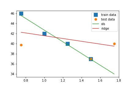
This is also how I generated the plot between the OLS model and the “imaginary” model at the start of this article. I think this plot shows the difference between OLS and ridge very well. Our training points very much represent the shape of a linear function. OLS regression takes full advantage of this and therefor generates a linear function that almost perfectly hits every training point. Ridge regression, however, also cares about small model weights, so it’s not as steep as the OLS model. The ridge line is a lot closer to our testing points than our OLS model is. Of course, we could take any combination of training and testing points. OLS would always generate the function with a minimal training error, while ridge would be a little bit more cautious. The result is that our OLS model has low bias and high variance, and our ridge model has a slightly higher bias, but a much lower variance. Ok! Now let’s tackle gradient descent.
Implementing Gradient Descent
We can reuse the gradient descent function that we’ve implemented in the article about Gradient Descent for Linear Regression. Here’s how the code looked like:
def gradient_descent(X, y, theta, criterion, number_of_iterations, learning_rate):X_b = add_intercept_ones(X)loss_history=[]for i in range(number_of_iterations):# predict and calculate lossf = create_function(theta) # create the current functiony_predicted = f(X_b) # predict our entire xloss = criterion(y,y_predicted) # calculate the errorloss_history.append(loss)# perform optimizationgradient = np.array([mse_derivative_b(y,y_predicted), mse_derivative_m(x,y,y_predicted)]) # calculate gradienttheta = theta - learning_rate * gradient #adjust m and bif i%10==0:print("Current Epoch: {}, Current Loss: {}".format(i,loss))return theta,loss_history
If this code doesn’t make a lot of sense to you, I recommend you give the article about Gradient Descent for Linear Regression, a try, as we build out this function step by step in that article.
Now we have to make some slight adjustments. First off we’ll have to define our new loss function and a new gradient function. Our loss is just the regular MSE with the added ridge penalty. So we can reuse our vectorized MSE implementation from the article Vectorization Explained, Step by Step and create a new function:
def mse(y, y_predicted):error = y-y_predictedloss = 1/(y.size) * np.dot(error.T, error)return lossdef ridgeMSE(y, y_predicted, alpha, theta):mse = mse(y, y_predicted)ridge_mse = mse(y, y_predicted) + alpha * np.dot(theta,theta)return ridge_mse
This is alright, but when we will later pass our ridgeMSE-function to our gradient descent algorithm,
we will somehow have to provide a value for alpha. We could use a default argument, but then we could
only pick one fixed value. Alternatively, we can pass in an argument for alpha to our gradient descent function.
Both of these methods are not extremely fun to work with, so what we’ll do instead is create a higher-order function
that will receive a value for alpha and return to us our ridgeMSE-function. It looks like this:
def getRidgeMSEFunction(alpha=0.0001):def ridgeMSE(y, y_predicted, theta):mse_loss = mse(y, y_predicted)ridge_loss = mse_loss + alpha * np.dot(theta,theta)return ridge_lossreturn ridgeMSE
Since our value for alpha won’t change during training, this approach works very well.
It might look a bit confusing at first because we are defining a function inside of a function,
but once you understand what’s going on, this approach can be quite handy.
Different Values for alpha.
You might be asking yourself why we set alpha=1 when we used the normal
equation and now we set alpha=0.0001 when using gradient descent.
The reason is that with the normal equation, we perform the entire computation
in one step, so our regularization parameter immediately affects every data point.
Also, every data point is only affected once.
With gradient descent, we solve our ridge regression iteratively. This means that at every iteration, we only want to apply a tiny bit of regularization, instead of applying it all at once.
An analogy would be cooking. Imagine you are making a soup and you want to add some seasoning to it. You have two options. You can either make a bold move and add all of your seasoning in at once, or you could cook the soup a bit, then add in a tiny amount of seasoning, taste it, add in some more, taste it, etc. But if you add in all of your seasoning at once, taste the soup, and then again add in the same amount of seasoning, your soup will not be very tasty. The seasoning would completely dominate the flavor of the soup, and the actual soup would not be able to present its taste very well anymore.
With our gradient descent algorithm, it’s quite similar!
If we would use gradient descent with alpha=1,
i.e. we were to add a large amount of seasoning at every iteration step,
we get the following model parameters: [16.578125 14.5625 ].
The regularization now dominates our loss and therefor our first model parameter is
not being able to grow as large as it should (to around 45), and it is instead
kept at a rather low value. This results in our second model parameter also having
to adjust to a suboptimal value.
This is also why the default value for alpha is 1 in scikit-learn’s Ridge-class,
but is only 0.0001 in scikit-learn’s SGDRegressor-class.
Now we’ll also have to define a function to compute our gradients. We can compute the gradient by differentiating our loss function, the ridge MSE. Our ridge-MSE looks like this:
Now, with the power of multivariable calculus we can compute:
I’ve used some colors to make the individual parts of the equation a bit clearer. The blue part (which includes the purple part) is our MSE. The purple part is our predicted y, which we can compute by multiplying our features with our model parameters . I’ve added a little in to signal that this already has intercept ones attached to it, to account for the bias, or intercept term. If you are confused as to why this is necessary and/or makes sense, I recommend you read this section of the article about linear regression. That part is not very long and in it, we will take a closer look at exactly this example, and how we can make sense out of it. If you’re struggling with the equation above, this should clear things up!
I don’t want to get into too much detail about this differentiation, because this is what you would do in a course about multivariable calculus. If you’re interested though, let me know and I’ll provide more info!
One small prettification we can do is add a factor of to our MSE, like so:
This will result in our gradient looking like this:
As you can see, the factor 2 is removed from our gradient. Oftentimes, in online courses or textbooks, you will see this being done to make the gradient a bit simpler. It does not really make that much of a difference since you can just increase or decrease to make up for the factor 2, but it’s still nice to know why this is sometimes done.
We can now directly translate our gradient into code. Because we also have to pass in an argument
for alpha, we can use the same approach as before:
def getRidgeGradientFunction(alpha=0.0001):def ridgeGradient(X_b, y, y_pred, theta):return -(2/y.size) * X_b.T.dot((y - y_pred)) + alpha * thetareturn ridgeGradient
With the loss and gradient now defined, we can implement our gradient descent algorithm!
We’ll make a slight change - our function will now receive an additional parameter gradient_function
which we will use to compute our gradient:
def gradientDescent(X, y, theta, criterion, gradientFunction, number_of_iterations, learning_rate):X_b = add_intercept_ones(X)for i in range(number_of_iterations):# predict and calculate lossf = create_function(theta) # create the current functiony_predicted = X_b.dot(theta) # predict our entire xloss = criterion(y, y_predicted, theta) # calculate loss# perform optimizationgradient = gradientFunction(X_b, y, y_predicted, theta) # compute gradienttheta = theta - learning_rate * gradient # adjust thetareturn theta
Let’s test our implementation:
theta_ridge_gd_1 = gradientDescent(X_train, y_train, theta, getRidgeMSEFunction(0.0001),getRidgeGradientFunction(0.0001), 1000, 0.03)print(theta_ridge_gd_1)# output: [44.41801778 -3.11386069]
Great, we get almost the same results as with our normal equation! We can make a small plot and compare our solution from the normal equation with the results of gradient descent:
plt.plot(X_train, y_train, "s", markersize=12, label="train data")plt.plot(X_test, y_test, ".", markersize=15, label="test data")plt.plot(X, X_b.dot(theta_ridge_gd_1), label="ridge gd")plt.plot(X, X_b.dot(theta_ridge_ne_1), label="ridge ne")plt.legend()plt.show()
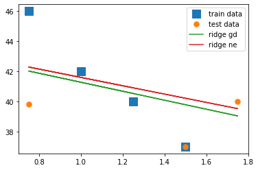
Nice! You could get even closer to the results from the normal equation by tuning the hyperparameters even more.
We can also solve ridge regression with gradient descent by using scikit-learn’s SGDRegressor-class.
Scikit-learn does a bit more under the hood, and to mimic our own function’s behaviour we’ll
have to pass a few additional parameters. For example,
SGDRegressor uses an adaptive learning rate by default.
To use a constant learning rate we pass the arguments learning_rate="constant"
and eta0=0.001. eta0 sets the initial learning rate.
We will also increase the maximum number of iterations to 10000.
We have to perform these adjustments because SGDRegressor
uses stochastic gradient descent (that’s where the S in SGD comes from),
while our own implementation uses regular gradient descent.
There are a couple of differences between the two variants,
but the most important one is that SGD does not converge as “cleanly”
as regular GD, but is computationally a lot less expensive.
With this we have:
sgdreg_ridge = SGDRegressor(penalty="l2", learning_rate="constant", eta0=0.001, max_iter=10000, random_state=42)sgdreg_ridge.fit(X_train,y_train)theta_ridge_gd_2 = np.array([sgdreg_ridge.intercept_[0], sgdreg_ridge.coef_[0]])print(theta_ridge_gd_2)# output: [43.1764243 -2.0467813]
Awesome, we get almost the same result as with our own implementation! We can again create a simple plot and check that our results are similar:
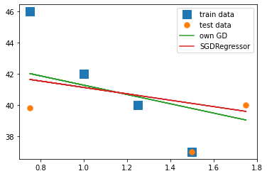
With scikit-learn’s SGDRegressor-class, if we train and evaluate it multiple times,
there will almost always be small differences in the final values,
because of the randomness involved in stochastic gradient descent.
This is why we provide an argument for random_state, to “fix” the randomness in our training and make
our results reproducible.
Visualizing Gradient Descent
Now that we’ve implemented gradient descent, let’s run the algorithm once more for ridge regression and visualize the results. Below you can see a 3-dimensional plot where for every combination of model parameters and (I’ve named them m and b in the plot, to make them more easily distinguishable), the ridge-MSE is plotted. By pressing the buttons at the top, you can perform one iteration step of gradient descent. After the first ten steps, each button press cycles through more than just one step at a time, so that you don’t have to press one button 300 times. Take a look and see how ridge regression converges.
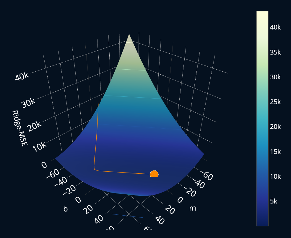
You might think that our algorithm overshoots the minimum and goes unnecessarily far to the “right”, but if you inspect the coordinates and loss values by hovering over the plot, you will actually see that the loss really does decrease in that direction. All in all, the visuals are not too surprising (which is good, because this means that our algorithm works as expected!), and look quite similar to the visualization we’ve performed for regular linear regression here. So everything looks alright! Time to round off this article and… wait. What is this next headline?
We Forgot Something Important
What? What are you talking about? Our gradient descent algorithm worked just fine, the solution was very close to the normal equation and we even visualized it in 3d and everything looked alright! What could we possibly forget?
Well, technically everything did go well. But in this example we were a bit.. lucky. Let’s take a look at what happens when we slightly modify our dataset. Right now our X tells us the age of every figure in years, right? Now what if we change that do days instead? In other words, we do this:
X_days = X * 365 # let's ignore leap years for now
Our dataset will still look the same and it will still hold the same information as before, but if we now run our OLS and ridge algorithms again, we get a different result. The model parameters for the original dataset, where our X represented the age of a figure in years, look like this:
print(theta_ridge_ne_1)# output: [44.36 -2.76]print(theta_ols_ne_1)# output: [ 54.3 -11.6]
Now we create new training and test splits X_days_train and X_days_test,
train our models in the exact same way we did before and our new model parameters are:
print(theta_ols_days_ne)# output: [54.3 -0.03178082]print(theta_ridge_days_ne)# output: [54.29968655 -0.03178006]
That’s right! Our ridge regression model has (almost) exactly the same model parameters as our OLS regression model! So the ridge regression penalty had no effect!
Ok.. that’s weird. What happens when we instead decide to let our X be the age of our figure in decades? Meaning we do this:
X_days = X / 10
We can now again create training and testing sets, train our models and we get:
print(theta_ols_decades_ne)# output: [ 54.3 -116. ]print(theta_ridge_decades_ne)# output: [41.29065421 -0.36137072]
Ok.. now the ridge parameters seem to go in the opposite direction. Let’s try to get some structure into these observations by plotting each of the OLS and ridge models on their respective datasets (click on the image to zoom in!):

Ok, much better! There are a few things we can see here:
- It seems that the ridge penalty becomes weaker when our data points are closer together, and stronger when they are further apart.
- The intercept term of the OLS models doesn’t change. Only the slope changes.
- The slope of the OLS models increases when our points are closer together.
Points 2 and 3 make sense together when we consider a simple example. Two data points from our original X were about 1 year apart from each other. Now the difference can be as high as 365 days! For us, those two mean exactly the same thing. But for our model, the numbers just increased by a factor of 365! Since our data points are now a lot further apart from each other, this also means that very small changes in our model parameters can drastically alter our loss. If we have two data points and , then our y-value will have changed by if we go from to . But if we have two data points and and we go from to , our y-value will have changed by ! This is why the slope of our OLS models increases when our data points are closer together from each other. Ok. Similarly, the slope decreases when our data points are further apart from each other. Makes sense, right? But what about ridge?
Take a look at the OLS model parameters for our X_decades. The slope is pretty high (in the absolutes),
it is around -116. Our ridge penalty penalizes large model weights, so our penalty hinders our
ridge model from developing such a high slope value. But our model parameters need
to be this large because our points are much closer together! This unlucky combination leads to our ridge
penalty completely taking over and our model looking like a flat line.
If we consider X_days, then our data points are very far apart, which means our model needs
smaller weights. But because our model parameters already are so small because of our scaling,
the ridge penalty does not see any problem whatsoever and does not penalize our model any further,
because the weights are already so small.
This issue appears very frequently in machine learning and it can be a real pain to deal with because you might not suspect that the scaling of your data is the leading cause for this issue. This issue also affects almost all regularized models, because they all share some sort of regularization term that punishes large model weights.
So what can we do about this? Is there any hope left for our ridge regression model? Yes, there is! And it is called standardization.
Originally I wanted to talk about standardization, what it is, why it can save our ridge regression model, and so on. But then this article got longer and longer and in the end, I decided to write a separate article all about standardization! After all, this article is already pretty long and I wanted to make a cut here so that you can process all of the information from this article, and then move onto the next one. So if you want to find out how you can save our ridge regression model from the pitfalls of different data scalings, head on to the article When You Should Standardize Your Data and learn all about the magic of standardization!
Finding the Optimal Value for
So far we’ve seen a number of examples that show ridge regression in action.
In the code examples, I’ve provided parameters for hyperparameters such as
the learning rate or . But the question is, how did I actually find
the right values for these hyperparameters? Do I just have a magical sense
that tells me which values will result in the lowest loss? Sadly, no.
The only way to find out the ideal values is to just try out a bunch of them
and then pick the ones that result in the best models.
This is called hyperparameter tuning. For , scikit-learn offers you
a built-in class called RidgeCV where you don’t have to provide an argument for .
Instead, multiple values of are tested using cross validation (That’s where the CV
in RidgeCV comes from) and the ideal one is chosen. You can specify the values for alpha
that should be compared to each other.
Below is an exemplary application of RidgeCV.
ridge_cv = RidgeCV(alphas=[0.1, 1.0, 10])ridge_cv.fit(X_train, y_train)print(ridge_cv.alpha_)# output: 0.1
As you can see, we compare the values 0.1, 1, and 10 for our hyperparameter alpha and then our
model just chooses the value for alpha that results in the best model!
Further Reading
If you have made it until the end of this article, great job! This was my most exhaustive article so far and I really hope that it could help you understand ridge regression better. Now you should be able to use regularization to further optimize your models and prevent them from overfitting. From here, there are two ways to continue learning.
Improving Regularization
As we saw before, ridge regression relies on an -parameter that helps control the regularization strength. But finding the optimal value for can be a bit tricky because it’s a hyperparameter. This is where the magic of hyperparameter optimization comes in! Hyperparameter optimization can optimize these values for you, and automatically select the values that result in the lowest losses and the best models. Hyperparameter optimization is extremely useful in practice, and if you want to learn more about it, I recommend that you read the article Hyperparameter Optimization Explained, Step by Step, where you will learn everything you need to know about this topic.
Another crucial aspect we’ve seen is just how important the scaling of your dataset is. Different scales can result in vastly different models, and not paying attention to the scaling of your data can cause a lot of pain and confusion. Luckily, there are ways to deal with this! One of these ways is standardization, which puts all of your data values onto the same scale. If you want to create reliable and consistent machine learning models with data on any scale, then you should read the article When You Should Standardize Your Data, where you will learn everything you need to know about standardization and how you can apply it in your own machine learning projects (Spoiler: It’s a lot easier than one might think!).
Ridge for Other Models
In this article, we looked at ridge regression, which is a regularized variant of OLS regression. But the ridge penalty is not just limited to plain old OLS regression! In fact, we can take most other linear models and just add the ridge penalty to its respective cost function! We can take the ridge penalty and apply it to models like logistic regression or polynomial regression. If you’re interested in these regularized models, I recommend you take a look at the articles Logistic Regression Explained, Step by Step and Polynomial Regression Explained, Step by Step respectively. In those articles you will learn everything about the named models as well as their regularized variants!
Share on:
