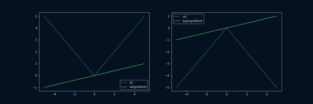
Subgradient Descent Explained, Step by Step
Gradient descent is one of the most popular algorithms to train machine learning models. However, many of the popular machine learning models like lasso regression or support vector machines contain loss functions that are not differentiable. Because of this, regular gradient descent can not be used. One of the most commonly utilized techniques to circumvent this issue is to use subgradients instead of regular gradients. And in this article, you will learn how it's done.
Share on:

Background image by Pontus Wellgraf (link)
Outline
You’ve probably heard about gradient descent. Maybe someone even told you that this or that machine learning model can be trained by using gradient descent. In many cases, what is actually used under the hood is not regular gradient descent, but subgradient descent. In this article, we will explore what subgradients are, how and why we can use them in practice, and what the potential dangers of subgradients are.
Prerequisites
Before reading this article, you should already be familiar with gradients and gradient descent. If you’re unfamiliar with gradient descent, don’t worry! Gradient descent is a lot less scary than it sounds, and it can be used for a variety of machine learning models, not just neural networks. If you’re interested in an introduction to gradient descent, check out the article Gradient Descent for Linear Regression Explained, Step by Step.
In this article, we will apply gradient descent to lasso regression, which is a slight variation of the popular linear regression algorithm. So if you want to understand that example fully, I recommend you take a look at Lasso Regression Explained, Step by Step.
With that being said, let’s get started!
The Problem
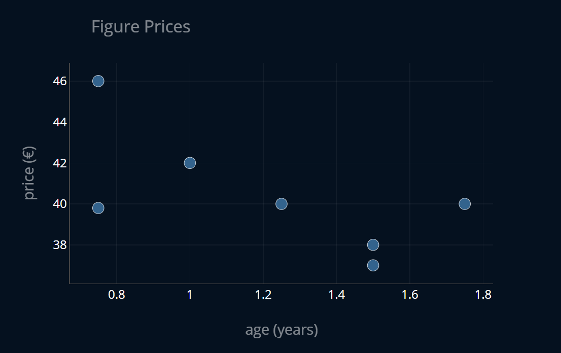
So why do we even need these subgradients? What’s the issue with regular gradients? For this, let’s look at a concrete example: lasso regression. Imagine we have a dataset of figure prices, where each entry in the dataset contains the age of a figure as well as its price for that age in € (or any other currency). We now want to predict the price of a figure given its age using lasso regression, to see how much the figures depreciate over time. The dataset looks like this:
We can now write down our lasso loss function like this:
where is the vector containing all of our model parameters. The term in blue is an L1-penalty, and it can be rewritten like this:
is an application of the absolute function, which looks like this:
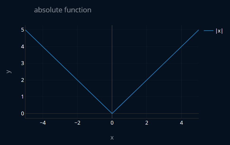
To find the optimal value for our model parameters we have to find the minimum of the . To find the minimum of a function, we usually have to take the first derivative of that function. In our case we have a multivariate function, so we will have to take the gradient of it. But here’s the problem: The L1 penalty inside of our is not differentiable at 0!
The slope of the absolute function is -1 for all of the negative values, and it is 1 for all of the positive values. But the slope at 0 is not defined!
Because of this, we can not differentiate our , and thus we can not find the model parameters for our lasso regression. Or can we?
Part 1: Subgradients
One key insight we can make is that the absolute function inside of our L1-penalty is only non-differentiable at zero. So maybe we can still differentiate our function at every point except 0, and then we’ll just find a clever way to solve the case when we get to the point at .
This is the first key insight into subgradients. What is a subgradient of a function at a point ? Well, if is differentiable at , then the subgradient is just the regular gradient of that function at that point . Ok, so far so good. But now comes the trickier part. What do we do when is not differentiable at ?
Let’s take a step back and visualize our absolute function again.
This time, I’ll also include the gradients for and .
Since we’re dealing with a univariate function the gradient
will just be a scalar. So instead of somehow adding this scalar into the plot,
what I will do is I will display the gradient as a linear function where the slope
of that function is exactly the value of the gradient, and the intercept is 0.
This may sound a bit confusing, so let’s jump to the visuals to make things more clear.
The plot below contains two gradients,
so feel free to toggle the visibility of the gradients by clicking on the labels
in the legend at the right part of the plot.
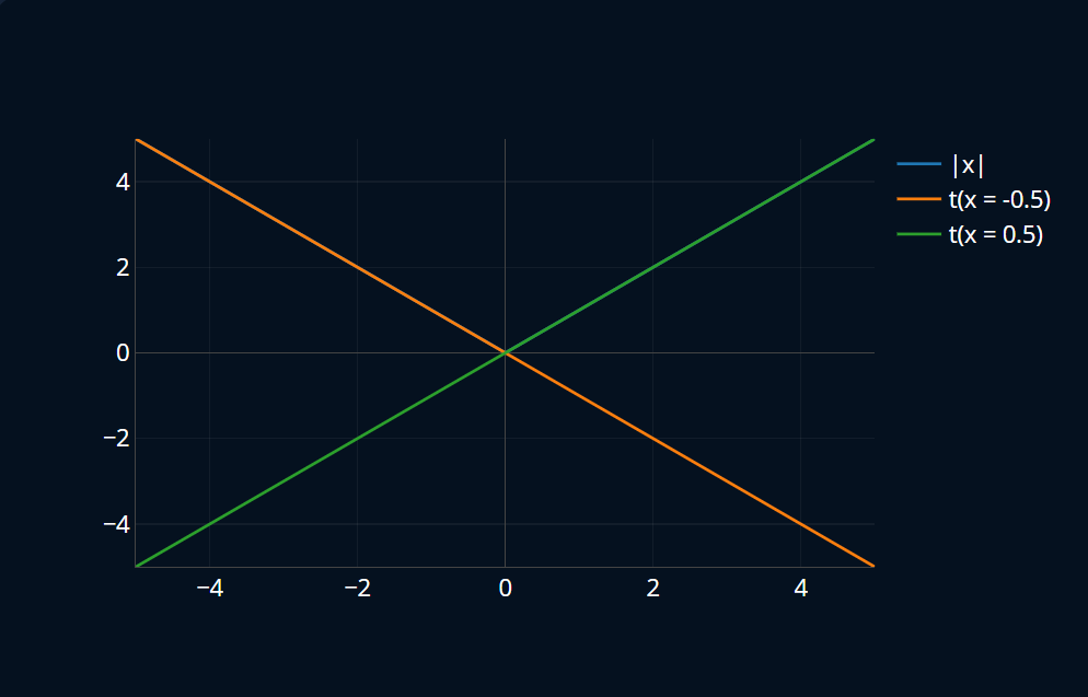
One thing you might notice is that the linear function represented by one of the two gradients is always either below or exactly on our main function . What’s even better is that this property holds true for all convex functions. What is a convex function? In a nutshell, a convex function is a function that has exactly one global minimum
Ok, so we know that gradients (or rather the linear functions we define around them) are so-called global underrestimators. Now if we’re going to define a subgradient of at 0, then it should probably look and behave somewhat similar to what a real gradient would look like at that point, if it existed in the first place. With this in mind, how could a potential subgradient of look like at ?
Since we can’t truly know how a real gradient would look like at that point, one idea is to look at the gradients in the neighborhood around 0, and then define the subgradient as an intermediate vector between the gradients around our non-differentiable point.
Right now this still sounds pretty vague, so below is a visualization showing many possibilities for an intermediate gradient at . At the bottom of the plot, there’s a slider which controls the value of the subgradient.
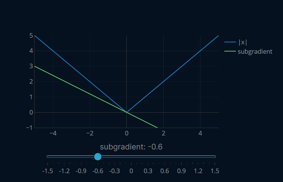
Notice how the line representing our subgradient turns orange once we cross the initial function, making the subgradient invalid because it would be greater than the neighborhood gradient, which is something we don’t want. Conveniently enough this also ensures that our subgradient is a global underrestimator of our function, just like a regular gradient would be. So any number between -1 and 1 (including both -1 and 1) is a valid subgradient for our function at .
That is also why subgradients are called subgradients. The prefix sub comes from Latin and means “below”, which makes sense now that we know that subgradients are global underrestimators, or in other words, lie below our function.
This is the second crucial insight into subgradients. They can be considered intermediate vectors of the neighborhood gradients, and they are global underrestimators of our function. This also means that there can be an infinite number of subgradients for a function at a non-differentiable point , which is in contrast to regular gradients, which are unique to every function and every point.
And that’s it! That is how subgradients are defined.
Formalizing Subgradients
Now let’s try to come up with a mathematical definition that encapsulates this behavior. Our definition might start like this:
So far so good! We’ve seen that subgradients are global underrestimators, so let’s try to come up with a mathematical way of writing this property down. At this point, you can pause for a second and think about how you would define this property.
An initial idea might look similar to this:
This says that the value of our subgradient at any point has to be lower than the value of our function at that same point . This definition seems intuitive, but let’s see if it really accurately describes what subgradients are. For this, we will look at the absolute function once again. Let’s create a plot where we will see the following things:
- the absolute function
- our subgradient of at the point
- for specific values of
- for specific values of
Since is a variable, we’ll add in a slider to control the value of . We’ll also consider just one fixed subgradient (namely 0.2), since, as we have seen before, the subgradient of the absolute function at can take on any value between -1 and 1. Here’s how that looks like:
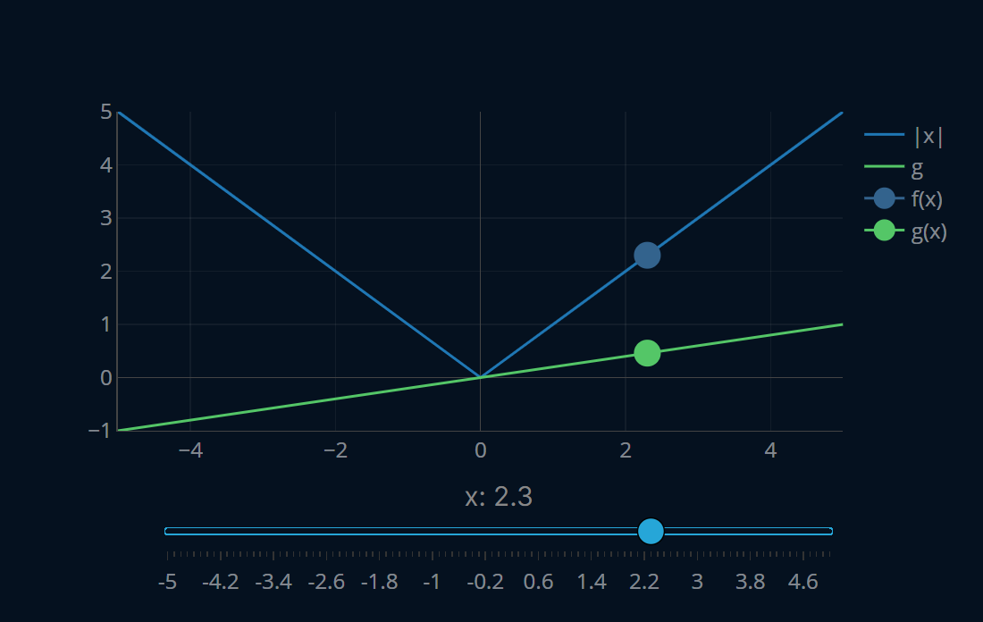
So far so good! We can see that is always greater or equal than .
Refining our Definition
Now let’s try a more complicated example. Consider the following function:
This function looks like this:
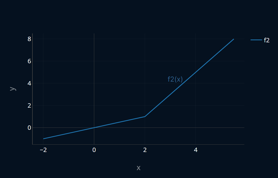
is not differentiable at , so let’s add in a subgradient at that particular point. The slope of is for every point less than 2, and 2 for every point after that. Since we can think of a subgradient as the intermediate vector between the gradients around it, a valid subgradient in this particular case should be 1. So let’s add the subgradient (once again represented as a linear function, we’ll call it ) to our plot and see how it looks like:
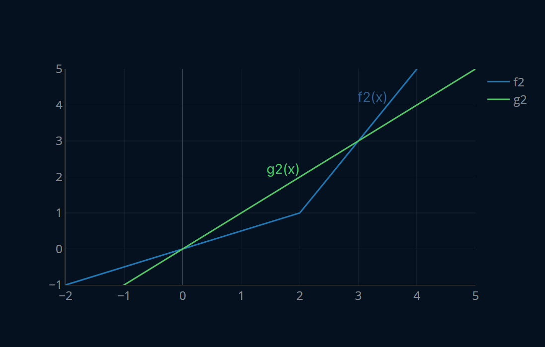
Well, that sure does not look as expected… our subgradient is at the wrong position! We want our subgradient to go through the point , but right now this isn’t the case. So what can we do? We can move our entire subgradient by to the right. Maybe you also remember from calculus that to move a function to the right by some amount, we counterintuitively have to subtract that amount from our function. So instead of calculating we will now calculate , which in our case will be . Now we have successfully shifted our function on the x-axis, but we still have to shift it on the y-axis. To do this we simply add to the right-hand side of our subgradient condition. In our particular case that would be .
Our subgradient definition now looks like this:
Ok, that seems reasonable. Let’s also visualize it to see if it actually does what we expect. Below is an interactive visualization where you can visualize the two steps we have just performed by pressing the button at the top of the plot.
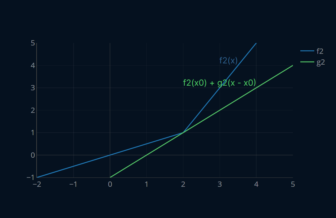
Much better! Now let’s look at the actual definition of subgradients and see how it compares to our own. Here goes:
A vector is a subgradient of a function at the point if for all points the following holds:
.
Personally, I find it a lot more intuitive to call and to call since this (at least for me) indicates that and lie on the same scale and that is really a variable whereas is just a single, fixed point. That is why I chose this version for this article, but I still wanted to show you this variant as well, since it is most common in literature.
Well if that doesn’t look familiar! The definition is pretty much exactly the same. The only difference is that the subgradient is transposed. This is necessary since our subgradient might live in more than just one dimension like in our example. Because of this, we have to transpose it to make the multiplication work. Apart from that our definition is exact, nice!
Now we understand where subgradients come from, why they’re useful and how they are defined. But you’re also probably interested in when they are actually used in practice. To answer this question, let’s look at subgradient descent!
Part 2: Subgradient Descent
Million-dollar question: what’s the difference between subgradient descent and gradient descent? That’s right, subgradient descent uses a subgradient instead of a regular gradient! That is the only difference between the two. However, subgradient descent might not work completely as expected in some cases, so it’s definitely worthwhile to implement subgradient descent and take a look at some potential weaknesses. For the implementation, we’ll reuse the code that we wrote in the article Gradient Descent for Linear Regression Explained, Step by Step. Here’s how the code looks like:
def gradient_descent(X, y, theta, criterion, gradient_function, number_of_iterations, learning_rate):X_b = add_intercept_ones(X)for i in range(number_of_iterations):# predict and calculate lossf = create_function(theta) # create the current functiony_predicted = f(X_b) # predict our entire xloss = criterion(y,y_predicted) # calculate the error# perform optimizationgradient = np.array( gradient_function(...) ) # calculate gradienttheta = theta - learning_rate * gradient #adjust m and breturn theta
add_intercept_ones is a little helper function that adds an additional column of ones to
our X to make calculations with the bias (or intercept) easier. You can find it’s
definition here.
create_function is another small helper, you can find it’s definition here.
Now all we need to do is rename our gradient to subgradient, like this:
def subgradient_descent(X, y, theta, criterion, subgradient_function, number_of_iterations, learning_rate):X_b = add_intercept_ones(X)for i in range(number_of_iterations):# predict and calculate lossf = create_function(theta) # create the current functiony_predicted = f(X_b) # predict our entire xloss = criterion(y, y_predicted) # calculate the error# perform optimizationsubgradient = np.array(subgradient_function(...)) # calculate gradienttheta = theta - learning_rate * subgradient # adjust m and breturn theta
Technically, you could even keep the old implementation altogether, since we only changed up
variable names. However this way I think it’s a bit easier to know just what exactly we’re doing.
Now that we have our general subgradient_descent-function defined, let’s look at a concrete example:
lasso regression.
Example Implementation: Lasso Regression
To recap, here’s how the loss-function of lasso looks like:
From our observations above we figured out that the subgradient of the absolute function at can be any number between -1 and 1, including -1 and 1. And for every other x, our subgradient is just the regular gradient, i.e. and . We can write this down like so
Does this function look familiar to you?
This looks pretty similar to the sign of the number . Any strictly positive number has sign 1, any strictly negative number has sign -1,
and for 0 we can just define that the sign is 0, which, conveniently, is a number between -1 and 1, and
even more conveniently is what np.sign(0) outputs.
With this we can now use the sign of as our subgradient, like so:
And that’s it! We have “fixed” our lasso-MSE and now it’s time to perform subgradient descent!
Implementing Subgradient Descent for Lasso
The only thing we have to implement now are our loss and (sub)gradient functions. In the article Ridge Regression Explained, Step by Step we’ve implemented these functions for ridge regression:
def get_ridge_mse_function(alpha=0.0001):def ridge_mse(y, y_predicted, theta):mse_loss = mse(y, y_predicted)ridge_loss = mse_loss + alpha * np.dot(theta, theta)return ridge_lossreturn ridge_msedef get_ridge_gradient_function(alpha=0.0001):def ridge_gradient(X_b, y, y_pred, theta):return -(2/y.size) * X_b.T.dot(y - y_pred) + alpha * thetareturn ridge_gradient
We can slightly modify this code to get our functions for lasso.
Instead of writing two new functions that return us our gradient and loss functions,
we’ll modify our existing ones to accept parameters alpha1 and alpha2 (or a1 and a2 for short)
that will control the lasso and ridge penalties respectively. With this,
we technically implemented functions not for lasso, but for elastic-net regression.
However, since elastic-net is just a linear combination of ridge and lasso,
this works out just fine.
With this we have:
def get_elastic_mse_function(a2=1, a1=0):def elastic_mse(y, y_predicted, theta):error = y - y_predictedreturn (1 / (y.size) * np.dot(error.T, error) # mse+ a2 * np.dot(theta, theta) # l2-penalty+ a1 * np.sum(np.abs(theta)) # l1-penalty)return elastic_msedef get_elastic_gradient_function(a2=1, a1=0):def elastic_gradient(X, y, y_pred, theta):return (-(2 / y.size) * X.T.dot(y - y_pred) # gradient of mse+ 2 * a2 * theta # gradient of l2-penalty+ a1 * np.sign(theta) # subgradient of-l1 penalty)return elastic_gradient
By calling get_elastic_mse_function with a1=0 and a2=0, we get the regular, unregularized MSE function.
With a2=0 we get the ridgeMSE and with a1=0 we get the lassoMSE. The same goes for our gradient function,
where we can just combine the penalties to prevent us from having to write three separate functions.
With the loss and gradient now defined, we can use our subgradient_descent-function like this:
subgradient_descent(X_train, y_train, theta,get_elastic_mse_function(a2=0, a1=1),get_elastic_gradient_function(a2=0, a1=1),number_of_iterations, learning_rate)
Here it is important to note that our X has to be standardized,
since we are using a regularized model.
If you’re unsure as to why this is truly necessary or what standardization
really is, I recommend you read Standardization Explained, Step by Step.
For now we will assume that our X was already standardized, to make the code more readable.
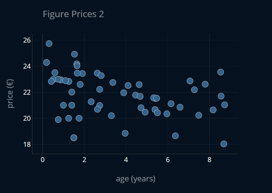
Also note that we are only using a portion of the dataset for our subgradient descent, a so-called training subset. You can read more about how to split your dataset correctly in the article How to Split Your Dataset the Right Way. For this article, we’ll already assume that our dataset has been split properly.
So let’s run lasso regression and see how it goes!
theta_lasso_subgd = subgradient_descent(X_train_s, # standardized!y_train,np.random.rand(2), # initialize theta as random vectorget_elastic_mse_function(a2=0, a1=1),get_elastic_gradient_function(a2=0, a1=1),1200,0.01,)print(theta_lasso_subgd)# output: [40.75 -2.74229857]
Alright, that looks good! If we train a regular OLS regression model then our model parameters will look more
like this: [41.25 -3.242]. So lasso did make our parameters a bit smaller, nice!
We can plot the two models and we get:
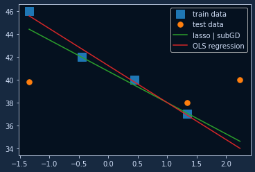
The lasso function is pretty similar to the regular linear regression function, just with slightly smaller coefficients. If we were to increase the L1-penalty coefficient, we would get an even more strongly regularized result.
The Fatal Flaw
The main property of lasso is that lasso is able to produce sparse model weights. In other words, lasso is able to set weights of unhelpful model parameters all the way to zero, unlike ridge regression for example. Since we’ve just implemented lasso regression, we should check whether our implementation zeroes out unnecessary weights, as we expect it to. We can do this by creating a random dataset (a random X and a random y) and then running lasso regression on it. Since the dataset is completely random, there should be no correlation between X and y, and thus lasso should set all of our model parameters to exactly zero. Let’s give it a try:
theta_rand = np.random.rand(51)X_rand = np.random.rand(100, 50)y_rand = np.random.rand(100)theta_rand_lasso_subgd = subgradient_descent(X_rand,y_rand,theta_rand,get_elastic_mse_function(a2=0, a1=1),get_elastic_gradient_function(a2=0, a1=1),3000,0.01,)print(theta_rand_lasso_subgd)# output similar to:# [ 0.01036144 0.00646848 0.00116589 0.00647136 -0.00524321 0.00290512# 0.00664798 0.00808131 0.00937785 0.00165406 -0.00257609 0.00490855# -0.00133889 -0.00582042 0.00832424 0.00403818 0.00799567 0.00062623# 0.01316767 -0.0043727 0.01226832 -0.0052027 0.00092482 0.00231925# 0.01305558 0.00906722 0.00154304 0.00505857 0.0087923 0.00346944# 0.00158308 0.0112326 -0.00631912 -0.0001088 -0.00211522 0.01203972# 0.00760454 0.01046682 0.00350387 -0.00540258 0.00655244 0.00841913# 0.00930862 0.00478768 -0.00475235 0.01260794 0.01329395 -0.00388777# 0.00920832 0.00485297 0.00296131]
Now I don’t know about you, but those values are not exactly zero. I mean sure, they’re close.
But lasso should be able to set them to exactly zero, and not just close to it.
That’s why we’re using it in the first place, right?
Even if we were to increase a1 and run subgradient descent again,
the parameters will still not be exactly zero.
Why is that so? Did we do something wrong? Surely there has to be a mistake in our code.
Surprisingly, no. Everything is working as intended.
When I first encountered this behavior, I did not know what caused the issue. So naturally, I started digging deeper and I also performed some experiments. The most common answer that I found online was that the problem lies in the subgradient. Since the subgradient is only an approximation of the real gradient
Now the question is, how often is this point at x = 0 hit? If you want to find this out for yourself, I recommend you take a look at the second programming exercise of the Reinforcement-section because that is exactly the purpose of that exercise. If you’re still reading, then you probably want to find out the answer. The answer is that the point at x = 0 is pretty much never hit. Why? The L1-penalty of is the sum of the absolute entries of , so for this term to be 0, every entry in has to be 0 as well. Or, in other terms:
The Fatal Flaw of…?
So if the subgradient is not the problem, then what is? The problem actually lies in gradient descent itself. The thing is, gradient descent in itself only approximates the optimal solution. In some cases, that approximation happens to be exactly the optimal solution. However, in our case, it is not. Why? Since there is no correlation between our randomized features, the optimal solution would contain only zeros, right? This means that as we get closer and closer to our optimal solution, our model parameters would get closer and closer to zero, but this also means that our gradient would shrink more and more! And with a smaller gradient, gradient descent will perform smaller and smaller updates. This means that we are asymptotically approaching the optimal solution and making smaller and smaller steps at every iteration. So to actually reach the exact optimal solution we would have to perform an infinite number of gradient descent iterations
We can see this even better when we visualize the values of over time. To do this, let’s generate a random dataset with only two entries, because visualizing 50-dimensional data is a bit tricky. We could either do this in 3D, where the first two dimensions would be the first and second value of , and the third dimension would be the lassoMSE for our randomized dataset. We will do this later when we visualize subgradient descent on our actual dataset, but for now a filled contour plot (or contourf plot) would be a better choice. A filled contour plot is a 2D plot where the background color is the third dimension. So in our example, the lassoMSE would be represented by the background color of the plot. If we track the value of at every iteration and plot it (in red) alongside our contourf plot, we get this:
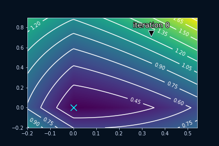
The dark region in the middle is where our loss is minimal. As we can see the point (0,0) lies exactly in that region. Now it might look like we pretty quickly reach our optimal point (0,0), but if we zoom in we will be able to better understand what really is going on:
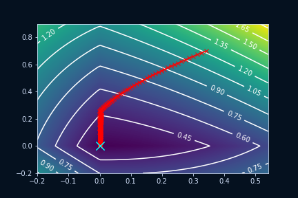
Our jumps around our optimal point, but it never reaches it exactly. Gradient descent is often explained as a traveler climbing down a hill, but here I think it makes sense to think of gradient descent as a game of golf, where is our golfball and the hole is our optimal solution. Putting the ball exactly into the hole is difficult as it requires good aim and just the right amount of force. But here, instead of a hole, the optimal point is just a marking on the ground. If putting a golf ball into a hole is difficult, then placing it onto a specific point on the ground is nearly impossible. That is why our (sub)gradient descent is hopping around the optimal point. It’s simply trying its best to get as close as possible to the optimum, but the ball keeps rolling just a bit further than it has to.
This is important because gradient descent (not stochastic gradient descent, but regular gradient descent) is oftentimes presented as an optimal solution finder, as I like to call it, even if it is a costly one. But this is simply not true as we see here. Usually, gradient descent finds a solution that is so close to the optimal one, that the difference is completely negligible. But if you are looking for some very specific values, like in the case of lasso, then this is an important fact to keep in mind, because it might explain some of the struggles you might encounter, similar to the ones presented in this article.
So now that we know about this issue, how can we solve it?
Fixing (Sub)gradient Descent for Lasso
This issue can actually be fixed rather easily.
The crucial part is that we know our weights will be set very close to zero,
even though they will not go all the way to zero.
So what we can do is we can add another parameter to our subgradient_descent-function
called epsilon, or eps for short. Then, at the end of an iteration of subgradient descent,
we will set all weights that are less than our eps to zero. So all we have to do is add this one line
to our subgradient_descent-algorithm:
def subgradient_descent(X,y,theta,criterion,subgradient_function,number_of_iterations,learning_rate,eps,):X_b = add_intercept_ones(X)for i in range(number_of_iterations):# predict and calculate lossf = create_function(theta) # create the current functiony_predicted = f(X_b) # predict our entire xloss = criterion(y, y_predicted) # calculate the error# perform optimizationsubgradient = np.array(subgradient_function(...)) # calculate gradienttheta = theta - learning_rate * subgradient # adjust m and btheta[theta < eps] = 0return theta
If we now run our subgradient descent on our random dataset again we get the following output:
theta_rand = np.random.rand(51)X_rand = np.random.rand(100, 50)y_rand = np.random.rand(100)theta_rand_lasso_subgd = subgradient_descent(X_rand,y_rand,theta_rand,get_elastic_mse_function(a2=0, a1=1),get_elastic_gradient_function(a2=0, a1=1),3000,0.01,0.01,)print(theta_rand_lasso_subgd)# [0. 0. 0. 0. 0. 0. 0. 0. 0. 0. 0. 0. 0. 0. 0. 0. 0. 0. 0. 0. 0. 0. 0. 0.# 0. 0. 0. 0. 0. 0. 0. 0. 0. 0. 0. 0. 0. 0. 0. 0. 0. 0. 0. 0. 0. 0. 0. 0.# 0. 0. 0.]
Awesome!
Visualizing Subgradient Descent
Now that we’ve fully implemented subgradient descent for lasso, let’s also visualize it! Before we used a filled contour plot to visualize how subgradient descent converges for a randomized dataset. Now we will do the same for our actual dataset of figure prices, but this time, we will use a 3D plot instead of a contour plot. The visualization will be similar to the one we created for ridge regression. At the top of the plot, there are buttons to control the current iteration of subgradient descent. Here’s how our algorithm performs:
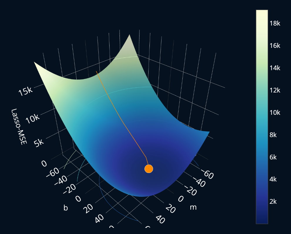
Nothing too special here, it looks mostly like regular gradient descent, and it also looks quite similar to the visualization we looked at earlier. But if we were to zoom in reeally deeply (deeper than this visualization allows us to), we would still see some jittering and imprecision, especially towards the end.
Here we can also intuitively see that the is convex because the surface plot representing the only has one minimum. This isn’t a mathematically rigorous proof, but for the intuition I think it conveys the message quite nicely.
Further Reading
Congrats on finishing this article! Hopefully, this article helped you understand what subgradients are, when and why they are used, as well as their strengths and weaknesses.
Subgradient descent is only one way to solve lasso regression, and there is in fact an even better way to solve lasso. It’s called coordinate descent and is extremely fast (convergence can often occur after just 2-3 epochs!). If you want to learn more about this fascinating algorithm and why it is so blazingly fast, I recommend you take a look at the article Coordinate Descent Explained, Step by Step, where you will learn everything you need to know about coordinate descent.
Maybe you have noticed that the L1-penalty can be written both as a sum as well as a vector operation. This is true not only for the L1-penalty but for most functions in machine learning! However, one of the two is clearly better than the other when it comes to performance. If you want to know which of the two variants you should prefer when implementing machine learning models, as well as why you should do so, check out the article Vectorization Explained, Step by Step.
Share on:

